Aggregation of objective functions

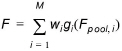
The defined objective functions are aggregated into one measure:

(1.10)   

where M is the number of objective functions that are aggregated, w_i, i = 1,2,..,M are the weights, and g_i(.), i = 1,2,..,M are transformation functions assigned to each objective function.

Three different transformation options are available:

No transformation:

(1.11)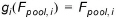   

Transformation to a common distance scale:

(1.12)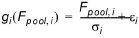   

where s_i is the standard deviation of the i'th objective function of the initial population used in the optimisation algorithm, and e_i is a transformation con­stant given by:

(1.13)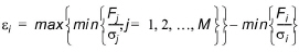   

Transformation to a common probability scale:

(1.14)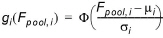   

where F(.) is the cumulative distribution function of the standard normal distri­bution, and m_i and s_i are the mean and the standard deviation of the i'th objective function of the initial population.

The transformation functions that are applied in the transformation to a com­mon distance scale and a common probability scale are introduced to com­pensate for differences in the magnitudes of the different measures so that all g_i(.) have about the same influence on the aggregated objective function near the optimum. When using a population-based optimisation algorithm, such as the Shuffled Complex Evolution method and the Population Simplex Evolu­tion, an initial population within the feasible region is evaluated. From this ini­tial population, the transformation functions are calculated.