
Routing is assigned to a river node and applied to flow leaving that river node. To add routing to a river node click on the append button
at the top of the table.
Then select the branch on which the river node is located and select the river node. To enable routing through an entire river branch, routing must be specified for all river nodes in that branch.
A number of routing options are available from a selection list. The below listed three routing options are supported by the Basin module:
Linear reservoir routing distributes flow leaving the river node over all time steps. When linear reservoir routing is selected a delay parameter K (the linear routing time lag), must be specified.
Delay parameter
The delay parameter K specifies the time for the incremental flood wave to traverse the river between the selected river node and the next downstream node. Its value may be estimated as the observed travel time of the flood peak between the nodes.
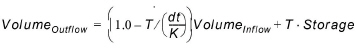
For a pulse inflow, outflow peaks after a specified time given by the time lag, and then decays exponentially. The formula used is:

where qo is outflow from the node, dt is time step length, qi is inflow to the node, s is storage in the subsurface, and K is the linear routing time lag (or delay parameter). T [-] is an intermediate result.
This algorithm includes damping. For a given time step, river storage is updated based on the following formula:. Variables dt, K and T are as explained previously.


Note that for linear reservoir routing, river storage is a virtual quantity that can be negative.
When selecting Muskingum routing a delay parameter K and a shape parameter X must be specified.
Delay parameter
The K parameter specifies the time for the incremental flood wave to traverse the river between the selected river node and the next downstream node. Its value may also be estimated as the observed travel time of the flood peak between the nodes.
Shape parameter
The shape parameter, X (dimensionless) depends on the shape of the modelled wedge storage. In natural rivers, X has a value between 0 (reservoir-type storage) and 0.3 with a mean value of 0.2 (X must always be less than 0.5 (full wedge storage)). Greater accuracy in determining X may not be necessary because the results are relatively insensitive to the value of this parameter.

Note that Muskingum routing can only be used when simulation time step length (dt) is within the following range: 2Kx < dt < 2K(1-x). If simulation time step length is outside this range Muskingum routing becomes unstable and is automatically replaced with linear reservoir routing. Linear reservoir routing is a special case of Muskingum routing with shape parameter x = 0. Unlike general Muskingum routing, linear routing is defined for all combinations of time step lengths and K values.
The Muskingum method is a commonly used hydrologic routing method for handling a variable discharge-storage relationship. This method models the storage volume of flooding in a river channel by a combination of wedge and prism storage. During the advance of a flood wave, inflow exceeds outflow, producing a wedge of storage. During the recession, outflow exceeds inflow, resulting in a negative wedge. In addition, there is a prism of storage, which is formed by a volume of constant cross section along the length of the prismatic channel.
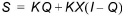
Assuming that the cross-sectional area of the flood flow is directly proportional to the discharge of the section, the volume of prism storage is equal to KQ, where K is a proportionality coefficient, and the volume of wedge storage is equal to KX(I - Q), where X is the shape parameter. The total storage S is therefore the sum of two components.
This expression can be rearranged to give the storage function for the Muskingum method:
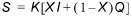
which represents a linear model for routing flow in streams.
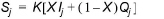
The values of storage at time j and j+1 can be written, respectively, as
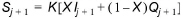
Using equations (6.6) and (6.7), the change in storage over time interval is:

The Wave translation algorithm basically uses a cyclical buffer with ‘slots’ for every time step. The inflow at a time step is put into the current slot, and the corresponding earlier inflow that was stored in that slot is pulled out. The index of the current slot cycles within the buffer, such that a new inflow always replaces the ‘oldest’ previous inflow. The number of slots in the buffer is equal to the number of time steps that a flow gets delayed with. The number of slots is computed as floor dt/K, where K can vary among reaches, and dt [time] is the simulation time step. The latter must be constant during a simulation; for months, a standard month length (30 days) is assumed.
Delay parameter
The K parameter specifies the time for the incremental flood wave to traverse the river between the selected river node and the next downstream node. Its value may also be estimated as the observed travel time of a distinct hydrograph peak between two nodes.
![]()