
Equilibrium Sorption Isotherms
The linear sorption isotherm is mathematically the simplest isotherm and can be described as a linear relationship between the amount of solute sorbed onto the soil material and the aqueous concentration of the solute:
(34.2)
where Kd is known as the distribution coefficient.
The distribution coefficient is often related to the organic matter content of the soil by an experimentally determined parameter (Koc) which can be used to calculate the Kd values.
(34.3) 
where foc is the fraction of organic carbon.
The retardation factor, R, is the ratio between the average water flow velocity (v) and the average velocity of the solute plume (vc). The retardation factor is calculated as
(34.4) 
The Freundlich sorption isotherm is a more general equilibrium isotherm, which can describe a non-linear relationship between the amount of solute sorbed onto the soil material and the aqueous concentration of the solute:
(34.5) 
where Kf and N are constants. Note that the units of Kf is a function of the units of c.
The relationship between K and N is shown in Figure 34.1.
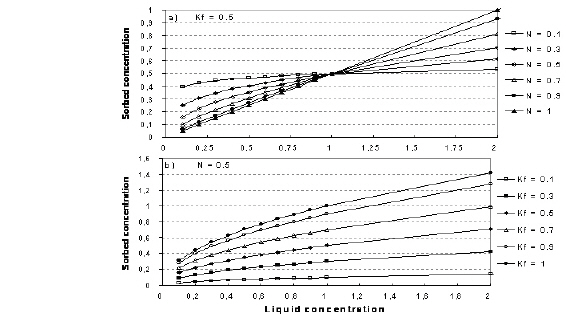
Figure 34.1 Illustration of the Freundlich isotherm. a) effect of change in N, b) effect of change in Kf
Both the linear and the Freundlich isotherm suffer from the same fundamental problem. That is, there is no upper limit to the amount of solute that can be sorbed. In natural systems, there is a finite number of sorption sites on the soil material and, consequently, an upper limit on the amount of solute that can be sorbed.The Langmuir sorption isotherm takes this into account. When all sorption sites are filled, sorption ceases. The Langmuir isotherm is often given as
(34.6) 
or
(34.7) 
where a is a sorption constant related to the binding energy and b is the maximum amount of solute that can be absorbed by the soil material. The relationship between a and b is shown in Figure 34.2.
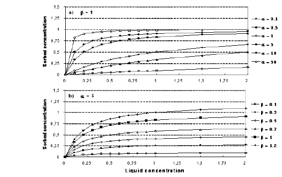
Figure 34.2 Illustration of the Langmuir isotherm. a) effect of change in a, b) effect of change in b.
![]()