Time step calculations

The time scales of the various transport processes are different. For example, the transport of solutes in a river is much faster than transport in the ground­water. The optimal time step is different for each component, where ‘optimal’ can be defined as the largest possible time step without introducing numeri­cal errors. In addition, the optimal time step varies in time as a consequence of changing conditions in the hydrological regime within the catchment.

Different time steps are allowed for the different components. However, an explicit solution method is used, which sometimes requires very small time steps to avoid numerical errors. The Courant and Peclet numbers play an important role in the determination of the optimal time step.

The user can specify the maximum time step in each of the components. However, the actual simulation time step is controlled by the stability criteri­ons, with respect to advective and dispersive transport, as well as the timing of the sources and sinks, and the simulation and storing time steps in the WM simulation.

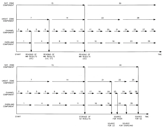
In Figure 33.2, you can see an example of the sequence of calling each com­ponents in the MIKE SHE advection-dispersion module. The time step in the river transport calculation is usually the smallest, whereas time step for groundwater transport is always the largest.

A transport simulation begins with the overland component followed by MIKE Hydro River, the unsaturated zone component and the groundwater compo­nent. Figure 33.2 shows how the simulation time steps can be controlled solely by the storing time step in the flow simulation.

Solute sources and the storing of data in the different components influences the time step. For example, in Figure 33.2, a SZ source requires that all com­ponents have a break when the source starts.

Figure 33.2        An example calculation sequence for solute transport in MIKE SHE.