Diffusive Wave Approximation

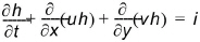
Using rectangular Cartesian (x, y) coordinates in the horizontal plane, let the ground surface level be z_g (x, y), the flow depth (above the ground surface be h(x, y), and the flow velocities in the x- and y-directions be u(x, y) and v(x, y) respectively. Let i(x, y) be the net input into overland flow (net rainfall less infiltration). Then the conservation of mass gives

(24.1)   

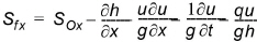
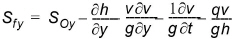
and the momentum equation gives

(24.2a)   

(24.2b)   

where S_f is the friction slopes in the x- and y-directions and S_O is the slope of the ground surface. Equations (24.1), (24.2a) and (24.2b) are known as the St. Venant equations and when solved yield a fully dynamic description of shallow, (two-dimensional) free surface flow.

The dynamic solution of the two-dimensional St. Venant equations is numeri­cally challenging. Therefore, it is common to reduce the complexity of the problem by dropping the last three terms of the momentum equation. Thereby, we are ignoring momentum losses due to local and convective acceleration and lateral inflows perpendicular to the flow direction. This is known as the diffusive wave approximation, which is implemented in MIKE SHE.

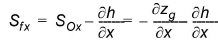
Considering only flow in the x-direction the diffusive wave approximation is

(24.3)   

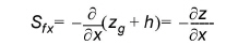
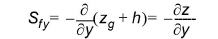
If we further simplify Equation (24.3) using the relationship z = z_g + h it reduces to

(24.4)   

in the x-direction. In the y-direction Equation (24.4) becomes

(24.5)   

Use of the diffusive wave approximation allows the depth of flow to vary sig­nificantly between neighbouring cells and backwater conditions to be simu­lated. However, as with any numerical solution of non-linear differential equations numerical problems can occur when the slope of the water surface profile is very shallow and the velocities are very low.

Now, if a Strickler/Manning-type law for each friction slope is used; with Strickler coefficients Kx and Ky in the two directions, then

(24.6a)   

(24.6b)   

Substituting Equations (24.4) and (24.5) into Equations (24.6a) and (24.6b) results in

(24.7a)   

(24.7b)   

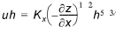
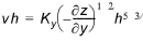
After simplifying Equations (24.7a) and (24.7b) and multiply both sides of the equations by h, the relationship between the velocities and the depths may be written as

(24.8a)   

(24.8b)   

Note that the quantities uh and vh represent discharge per unit length along the cell boundary, in the x- and y-directions respectively.

Also note that the Stickler roughness coefficient is equivalent to the Man­ning M. The Manning M is the inverse of the commonly used Mannings n. The value of n is typically in the range of 0.01 (smooth channels) to 0.10 (thickly vegetated channels), which correspond to values of M between 100 and 10, respectively.