Governing equations

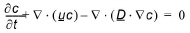
The transport of solutes and particle tracking in the saturated zone is gov­erned by the advection-dispersion equation, which for a porous medium with uniform porosity distribution is formulated as:

(37.1)   

where c is the solute concentration, t is time,  is the groundwater pore velocity, and is the dispersions tensor. In the particle model a large num­ber of particles are moved individually in a number of time steps according to contributions from advective and dispersive transport. A particle mass is associated to each particle, which means that the number of particles in a cell corresponds to a solute concentration.

For isotropic conditions in the soil matrix the displacement of a particle is described by the following equation [Thompson et al., 1987].

(37.2)   

where  is the particle co-ordinates,  is the time step length,  is a vector containing three independent random numbers equally distributed in the interval [-1, +1] and

(37.3)   

where

(37.4)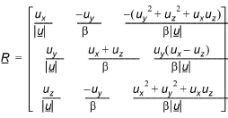   

(37.5)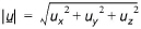   

(37.6)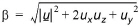   

(37.7)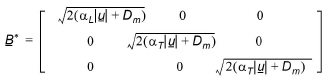   

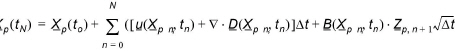
a_L and a_T are the longitudinal and transversal dispersion coefficients, respec­tively and D_m is the neutral dispersion. Using (37.2) repeatedly, the location of a particle at time t_N=NDt can be determined:

(37.8)   

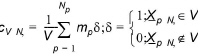
After applying (37.8) for a large number of particles, (i.e. N_p), the average sol­ute concentration for an arbitrary volume can be calculated using (37.9)

(37.9)   

where m_p is the particle mass. Using this procedure an accurate solution of the advection-dispersion equation (37.1) can be obtained [Thompson et al., 1987; Thompson and Dougherty, 1988; Kitanidis, 1994].

The term  in (37.2) and (37.8) is assumed to be much smaller than the remaining term and is omitted for the benefit of the computational speed. This may, however in some situations result in an accumulation of particles near boundaries or stagnation points. [Kinzelbach and Uffink, 1989; Uffink, 1988; Kitanidis, 1994].

Prior to the particle tracking calculations the transient three-dimensional ground water flow field must be calculated. The groundwater velocities are used by the particle model to calculate  using linear interpolation for the spatial interpolation in the three directions in the grid cells. For time integration, simple Eulerian integration is used. The numerical input used by the water movement calculations is reused in the particle model as control volumes (see (37.9)) and for the specification of initial and boundary condi­tions.

The vertical position of the particles is corrected for changes in cell thickness when a particle moves horizontally from one cell to the next. The correction uses the relative vertical location at the old location to determine the new ver­tical location:

(37.10)   

where old indicates the previous cell and new the current cell. The correction is only applied when moving horizontally from one cell to the next i.e. there is no interpolation of layer thickness during the movement within a single cell. This results in sudden changes in the vertical location at cell boundaries.

The following particle sinks can remove particles from model cells:

·         constant concentration boundary receiving particles

·         well

·         river

·         drain connected to a river or the boundary

·         exchange to the unsaturated zone

·         constant concentration source with a lower concentration than the calcu­lated concentration

The following particle sources can add particles to model cells:

·         constant concentration boundaries

·         a solute concentration in precipitation

·         a source in the saturated zone with a specified mass inflow rate

·         a constant concentration source with a higher concentration than the cal­culated concentration

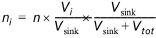
The PT module only calculates particle movements in the saturated zone. However, the volume of water removed by the wells, rivers, drains and the unsaturated zone is known. This volume of water is used to calculate the number of particles that are removed by each of the sinks using the formula:

(37.11)   

where n_i is the number of particles removed by sink i, n is the number of par­ticles in the saturated zone, V_i is the volume of water exchanged with sink i, V_sink is the volume of water exchanged with all sinks, V_tot is the total volume of water in the saturated zone.

Equation (37.11) is used to calculate the number of particles, which should be removed by each sink at each time step. This is, however, not necessarily a whole number of particles. The PT module takes care of this by retaining all the fractions of particles from previous time steps until it can remove a whole particle. Particles are always assigned one by one to the sinks, with prefer­ence given to the sink in need of most particles. In case there is more than one sink in a cell, with each of these sinks requiring the same number of par­ticles, there is a random assignment of one particle to one of these sinks. If there are any more particles left after this assignment, the next particle will then go to one of the other sinks.

Constant concentration sources and sinks at boundaries or inside the model domain are handled by calculating the number of particles that corresponds to the concentration and truncating this value to a whole number. For the mass flux source and the precipitation source the concentration is again con­verted to a number of particles. The whole number obtained by truncating this value is added to the compartment containing the source. The fractions that are left over after truncation are accumulated until a whole number of parti­cles has been attained in one of the next time steps at which time an addi­tional particle is added to the compartment in which the source is located.

Drains remove particles to rivers or to the boundary out of the model domain. Drains can also transfer particles internally in SZ. If this occurs the particles are moved from one compartment to another by the drain. Note that there is no time lag in this process.

To trace the particles, calculate transport times, capture zones, groundwater age, etc. each particle is associated with a particle ID, model time and loca­tion at which the particle was introduced in the model (time and co-ordinates of 'birth'). When particles enter sinks or are introduced into the model domain by a source, this information is registered together with the source/sink type and the registration time and location before removing or adding the particle. The registration process is also used for keeping track of particles that enter registration cells. A particle is only registered the first time it enters a registra­tion cell. This avoids repeated registration of particles that have entered a registration cell and which are not (immediately) removed by a sink.