The MIKE SHE allows for flow through drains in the soil. Drainage flow occurs in the layer of the ground water model where the drain level is located. In MIKE SHE the drainage system is conceptually modelled as one 'big' drain within a grid square. The outflow depends on the height of the water table above the drain level and a specified time constant, and is computed as a linear reservoir. The time constant characterises the density of the drainage system and the permeability conditions around the drains.
The drainage option may not only be used to simulate flow through drainpipes, but also in a conceptual mode to simulate saturated zone drainage to ditches and other surface drainage features. The drainage flow simulates the relatively fast surface runoff when the spatial resolution of the individual grid squares is too large to represent small scale variations in the topography.
Drainage water can be routed to local depressions, rivers or model boundaries. See Groundwater drainage (V1 p. 61) for further details about routing of drainage water.
There are also some additional Extra Parameter options for drainage routing:
· SZ Drainage to Specified MIKE Hydro River H-points (V1 p. 758)
· SZ Drainage Downstream Water Level Check (V1 p. 761)
· Time varying SZ drainage parameters (V1 p. 761)
· Time varying SZ drainage parameters (V1 p. 761)
· Canyon exchange option for deep narrow channels (V1 p. 764)
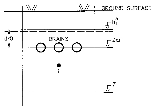
Figure 30.7 Schematic presentation of drains in the drainage flow computations.
SZ Drainage with the PCG solver
When the PCG solver is used, the drain flow is added directly in the matrix calculations as a head dependent boundary and solved implicitly, by
(30.22) 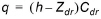
where h head in drain cell, Zdr is the drainage level and Cdr is the drain conductance or time constant.
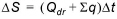
When the SOR solver is used, drainage is only allowed from the top layer of the saturated zone model. In this case, the new water table position at the end of the time step is calculated from the flow balance equation
where DS is the storage change as a result of a drop in the water table, Qdr is the outflow through the drain and Sq represents all other flow terms in a computational node in the top layer (i.e. net outflow to neighbouring nodes, recharge, evapotranspiration, pumping and exchange to the river etc.).
The change in storage per unit area can also be calculated from
where d0 is the depth of water above the drain at the beginning of the time step, dt is the depth of water above the drain at the end of the time step and Sy is the specific yield.
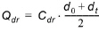
Qdr is calculated based on the mean depth of water in the drain during the time step. Thus,
where Cdr is the drain conductance or time constant.
Substituting (30.24) and (30.25) into (30.23) and rearranging, the water depth at the end of a time step, dt, can be calculated by
(30.26) 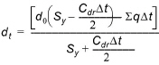
From which the new water table elevation, ht, at the end of the time step can be calculated by
(30.27) 
where Zdr is the elevation of the drain.
The drainage outflow is added as a sink term using the hydraulic head explicitly. The computation for drainage flow uses the UZ time step, which is usually smaller than the SZ time step. The initial drainage depth d0 at the beginning of an SZ time step is set equal to h - Zdr, where h is the water table elevation at the end of the previous SZ time step. d0 is adjusted during the sequence of smaller time steps so that a successive lowering of the water table and the outflow occurs during an SZ time step. This approach often overcomes numerical problems when large time steps are selected by the user. If the drainage depth becomes zero during the calculations drainage flow stops until the water table rises again above the drain elevation.
![]()