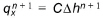
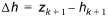
from neighbouring nodes and source/sinks between time n and time n+1 is given by:
The Successive Overrelaxation (SOR) Solver
Equation (30.1) is solved by approximating it to a set of finite difference equations by applying Darcy's law in combination with the mass balance equation for each computational node.
Considering a node i inside the model area, the total inflow from neighbouring nodes and source/sinks between time n and time n+1 is given by:
where  is the volumetric flow in vertical direction,
  is the volumetric flow in horizontal directions, R is the volumetric flow rate per unit volume from any sources and sinks, Dx is the spatial resolution in the horizontal direction and Hi is either the saturated depth for unconfined layers or the layer thickness for confined layers. See Figure 30.3 and Figure 30.4 for a description of the geometric relationships between the cells.
The horizontal flow components in Eq. (30.14) are given by
where C is the horizontal conductance between any of the adjacent nodes in the horizontal directions.
The horizontal conductance in Eq. (30.15) is derived from the harmonic mean of the horizontal conductivity and the geometric mean of the layer thickness. Thus, the horizontal conductance between node i and node i-1 will be
(30.16) 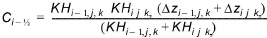
where, KH is the horizontal hydraulic conductivity of the cell and Dz is the saturated layer thickness of the cell.
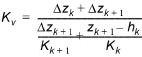
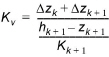
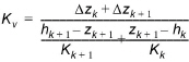
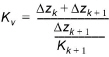
The vertical flow components in Eq. (30.14) are given by
(30.17) 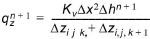
where Kv is the average vertical hydraulic conductivity between nodes in the vertical direction, and Dzi,j,k and Dzi,j,k+1 are the saturated thicknesses of layers k and k+1 respectively. For the average vertical hydraulic conductivity, Kv, the SOR solver distinguishes between conditions where the hydraulic conductivity of layer k is greater than or less than the hydraulic conductivity of layer k+1. These cases are shown in Table 30.1 and Table 30.2.
|
|
Layer k |
||
|---|---|---|---|
|
confined |
unconfined |
||
|
Layer k+1 |
confined |
|
|
|
unconfined |
|
|
|
|
|
|
||
|
|
Layer k |
||
|---|---|---|---|
|
confined |
unconfined |
||
|
Layer k+1 |
confined |
|
|
|
unconfined |
|
|
|
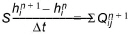
The transient flow equation yields the finite difference expression
where S is the storage coefficient and Dt is the time step. Eq. (30.18) is written for all internal nodes N yielding a linear system of N equations with N unknowns. The matrix is solved iteratively using a modified Gauss Seidel method (Thomas,1973).
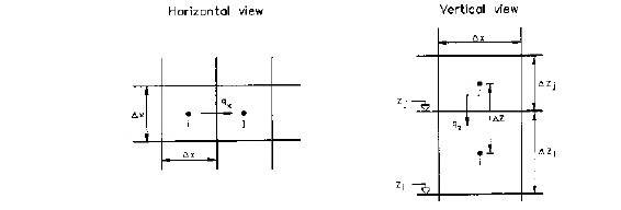
Figure 30.3 Spatial discretisation.
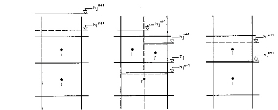
Figure 30.4 Types of vertical flow condition, a) confined conditions in nodes i and j, b) unconfined condition in node i, c) unconfined in nodes i and j, d) dry conditions in node j and confined conditions in node i.
![]()