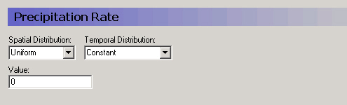
If the time-varying Real parameter does not vary spatially then the parameter must be defined as Global with either a Fixed or Time-varying value (see Uniform + Constant and Uniform + Time Varying).
Often, time-varying data, such as precipitation rate, are spatially distributed using measurement stations, which in the model are translated into model zones using, for example, Thiessen polygons. In this case, each station is associated with a .dfs0 time series file that contains the time series of precipitation rate. Station-based zones are defined using Integer Grid Codes in either a .dfs2 file as Grid Codes, or in a Shape (.shp) file as polygons with an Integer Code (see Station-based + Grid Codes or Polygons).
The parameter Value will be assigned to every cell in the model or layer as appropriate and will remain constant throughout the simulation.
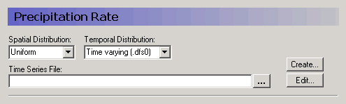
The time series in the .dfs0 file will be assigned to every cell in the model or layer as appropriate.
Station-based + Grid Codes or Polygons
Station-based time varying data means that the model domain is divided into zones that are defined by an Integer Grid Code.
If a .dfs2 file is used, then the Integer Grid Codes are defined on a regular grid, which is interpreted to the model grid during the Pre-processing stage.
If the Integer Grid Codes are defined using polygons then you must supply an ArcView .shp file containing polygons each with an Integer Grid Code. The item Fill Gaps with: allows you to define the Integer Grid Code to use in the event that a cell is not included within one of the polygons.
Once the file containing Integer Grid Codes has been defined, a new level in the data tree will appear below the current level, containing one entry for every unique Integer Grid Code in the file.
On this level, you must then supply a time series values for every Integer Grid Code. However, the time series can also be fixed, in the sense that a constant value over time is used. This makes it easy to use detailed time series for some zones and constant values for zones where little information exists.
The time series dialogue itself includes two graphical views. The upper graphic displays the time series that is being applied and the lower graphic shows where the time series will be applied.
![]()