Sigma

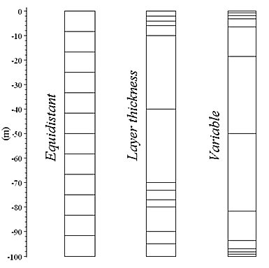
In the sigma domain the vertical distribution of the layers can be specified in three different ways:

·         Equidistant

·         Layer thickness

·         Variable

Figure 5.4           Examples of vertical distribution of layers for a water column 100 m deep. A number of 12 layers has been applied for all three options.
Left column: Equidistant distribution
Middle column: Layer thickness distribution
Right column: Variable distribution

For all three options you must specify the number of vertical layers (ele­ments).

Selecting equidistant distribution, the layers are distributed equidistant across the water depth.

Selecting layer thickness distribution, the fraction of each layer’s thickness across the water depth must be specified. Note that the sum of the values for the layer thickness must be equal to 1.

Selecting variable distribution, you must specify three vertical distribution parameters:

1.       sigma_c (s_c )
s_c is a weighting factor between the equidistant distribution and the stretch distribution. The range is

. The value 1 corresponds to equidistant distribution and 0 corresponds to stretched distribution.
A small value of s_c can result in linear instability.

2.       theta (q )
q is the surface control parameter. The range is

.

3.       b is the bottom control parameter. The range is

.

The variable s-coordinates are obtained using a discrete formulation of the general vertical coordinate (s-coordinate) system proposed by Song and Haidvogel (1994).

If q <<1 and b=0 an equidistance vertical resolution is obtained. By increasing the value of q , the highest resolution is achieved near the surface. If q >0 and b=1 a high resolution is obtained both near the surface and near the bottom.

A detailed description of the equations behind the variable distribution can be found in the scientific documentation for MIKE 21 & MIKE 3 Flow Model FM, Hydrodynamic and Transport Module.

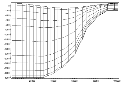
Figure 5.5           Example of vertical distribution using layer thickness distribution. Num­ber of layers: 10, thickness of layers 1 to 10: 0.025,0.075,0.1,0.1,0.2,0.2,0.1,0.1,0.075,0.025

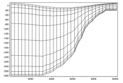
Figure 5.6           Example of vertical distribution using variable distribution. Number of layers: 10, sigma_c = 0.1, theta  = 5, b = 1