Standard deviation

The dialogue enables definitions of standard deviation specifications, which are used in the specific perturbation definitions at boundary locations in the model.

Standard deviations are added or deleted using the Append ‘+’ or Delete ‘-’ buttons above the overview table.

Standard deviation

ID. Identification name of the standard deviation.

Data type. The data type to which the standard deviation may be applied. Only the standard deviations with the appropriate data type can be selected for a given perturbation, depending on the data type the perturbation is applied to.

Type. The standard deviation may be of three different types:

·         Constant. The user specifies a constant value.

·         Relative. The standard deviation is taken as a relative value of the boundary condition. Note that the percentage is applied to the absolute value, when the data type is discharge, wind velocity, wind direction, pre­cipitation, temperature, salinity or concentration. When updating on water level, the percentage is interpreted as being with respect to the water depth.

·         Time varying. The standard deviation may vary with time with the varia­tion defined in a time series file.

Value. The value used as constant or relative standard deviation.

File. The time series containing the time varying standard deviation. The but­ton to the right may be used to either browse, create, edit or plot the time series.

Item. This field shows the name of the item selected in the time series.

Time constant before TOF. The time constant should be interpreted as the time it takes for the correction to drop to half the initial magnitude (exponential decay). The errors applied at the boundaries may be described through a first order auto regressive process:

where

x_n         the error at time step n

f         the regression coefficient

e         white noise

The regression coefficient should be interpreted as the ‘memory’ of the model error. To ensure that this ‘memory’ is independent of the time step used the user is required to specify a time constant instead. The relation between the regression coefficient and the time constant is:

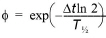
where

Dt   the simulation time step

ln   the logarithm with base e.

T_½   the time constant TC.

The numerical value of the regression coefficient must be less than unity to ensure that the variance of the model error is limited. A negative time con­stant results in a regression coefficient which is greater than unity.

The model errors being described through the auto regressive process are used in the forecast period to generate errors to be added to the boundaries. If the forecast is deterministic, the model errors are described through the auto regressive process without adding white noise. The model errors fade out according to an exponential decay.

Time constant after TOF. See description above for Time constant before TOF.

Apply lower limit. When applying a relative or time varying standard devia­tion, the user may apply a lower bound on the standard deviation, by activat­ing this option. The lower limit must then be specified in the Value field to the right.

Apply upper limit. When applying a relative or time varying standard devia­tion, the user may apply an upper bound on the standard deviation, by acti­vating this option. The upper limit must then be specified in the Value field to the right.