The update parameters page defines model locations where model updating is to be done. It is used for both the updating with weighting function and with Kalman filter.
Update definitions (i.e. updated points in the model) are added or deleted using the Append ‘+’ or Delete ‘-’ buttons above the overview table at the bottom of the dialog.
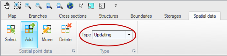
Note that update points can also be added, edited and deleted from the map, using the ‘Updating’ type of data in the Spatial data ribbon in Map view (see Figure 14.1).
Figure 14.1 Map view ribbon for inserting and editing updates
Each update definition represents a location where observed data are available and where the model is going to be updated. The simulation will actually be updated only for locations where the 'Include observation for model updating' is active. When this option is not selected, the update definition is ignored during the simulation. To define an observation location, the parameters below have to be specified.
Location
ID. String identification of the update definition.
Branch name. The name of the branch where observation data is located. It can be chosen from the drop down list.
Chainage. Chainage within the branch where the observed data are located. The chainage does not have to coincide with the location of a calculation point since MIKE HYDRO uses a linear interpolation for determining the simulated value at the appropriate measurement location.
Updated item. The type of variable on which the update is performed. Depending on the modules included in the simulation (in the Modules page), the type can be either a water level, a discharge or an AD/WQ component.
AD / WQ component. The component to be updated must be selected from the list of components either defined in the Advection-Dispersion module or derived from the list of state variables from the Water Quality module.
Observed data
Time series file. The time series file containing the observed data. File selection button ‘…’ may be used to either browse, create, edit or plot the time series.
Item. This field will present the name of the item selected in the time series.
Weighting function parameters
The weighting function parameters are visible when data assimilation mode is ‘updating with the weighting function’.
A weighting function definition must be specified for each update definition with the main purpose of defining how model corrections at the measurement location are distributed to neighbouring calculation points in the river network.
Distribution type. Three different types of weighting functions are available:
· Constant: in this case the error correction is distributed evenly over the grid points between the specified upstream and downstream chainages.
· Triangular: in this case the error correction is linearly decreasing from a maximum correction at the measurement location (specified in the ‘Location’ part) to 0 at the upstream and downstream chainages.
· Mixed exponential: in this case the error correction is decreasing according to an exponential function from a maximum correction at the measurement location to the upstream and downstream chainages, where the correction is about 0.01 times the correction at the measurement location.
Amplitude. The amplitude specifies the fraction of the observed error at the measurement location that should be applied as error correction at that point. The amplitude should reflect the confidence in the observation as compared to the model forecast. That is, if the amplitude equals one, the measurement is assumed to be perfect, whereas for smaller amplitudes, less emphasis is put on the measurement as compared to the model forecast.
Upstream chainage. It represents the upstream extent of the reach where the weighting function is applied (in the branch where the measurement point is located).
Downstream chainage. It represents the downstream extent of the reachwhere the weighting function is applied (in the branch where the measurement point is located).
Include connected branches. If this option is selected, the correction is also applied to tributaries (if any) which are connected to the main river between the specified upstream and downstream chainages. The correction is applied within the same extent and with the same amplitude and distribution as for the branch where the measurement is located.
Soft start. Number of time steps used to fade up the correction initially, starting from zero correction at the first updated time step up to full correction after the fade-up period. This function helps avoiding model instabilities since the error correction value is applied gradually rather than abruptly.
Error forecast
The error forecast parameters are visible only when performing updating with the weighting function. The error forecast definition includes two parameters:
· Include. The weighting function update procedure up to Time of Forecast may be combined with error forecasting at updating points, in the forecast period (i.e. after the time of forecast). This option is applied when the ‘Include’ box is checked. Error forecasting is mandatory and always included, when updating on discharge measurement.
· In that case, an equation defining how the calculated error function is forecasted over time must be selected in the drop-down list. The error function is derived during simulation in the updating period (up to Time of Forecast). Forecast Equations are defined in the ‘Equation’ tab.
The forecasted error correction is also distributed to the neighbouring points. Thus, by applying error forecasting, the model is updated also in the forecast period, with respect to the selected equation.
Standard deviation
A Standard deviation parameters group box is visible when performing updating with the Kalman filter only. The standard deviation must be specified for each update definition.
Type. The standard deviation may be of three different types:
· Constant. The user specifies a constant value.
· Relative. The standard deviation is taken as a relative value of the measurement. Note that the percentage is applied to the absolute value, when the updated item is a discharge or component. When updating on water level, the percentage is interpreted as being with respect to the water depth.
· Time varying. The standard deviation may vary with time with the variation defined in a time series file.
Value. The value used as constant or relative standard deviation.
File. The time series containing the time varying standard deviation. The button to the right may be used to either browse, create, edit or plot the time series.
Item. This field shows the name of the item selected in the time series.
Apply lower limit. When applying a relative or time varying standard deviation, the user may apply a lower bound on the standard deviation, by activating this option. The lower limit must then be specified in the Value field to the right.
Apply upper limit. When applying a relative or time varying standard deviation, the user may apply an upper bound on the standard deviation, by activating this option. The upper limit must then be specified in the Value field to the right.

Important: When updating is applied, the model state is updated using observed data up to the time of forecast. After Time of Forecast, forecasting is performed either using the error prediction model (if an equation has been defined), or for kalman filter updating either using a stochastic or deterministic forecast.
This functionality therefore assumes that observed data are available up to the time of forecast. In case observed data are missing before the time of forecast, the simulation will still run, but the following rules will apply:
· If observed data are missing at the beginning of the simulation, the updating will only start at the time when observed data become available
· If the model is being updated and if some observed data are missing before the time of forecast, the error prediction model will be applied
· If some observed data are available before the time of forecast but not sufficiently to compute the error prediction, or if no observed data at all is available before the time of forecast, then the update location is fully disabled during the simulation. That is, no update or error prediction is performed at this location.
![]()