Maps

Maps

The ‘Maps’ page may be used to produce two dimensional maps based on the one-dimensional simulations from MIKE HYDRO River. The maps are saved in dfs2 files (rectangular grids) and constructed through interpolation in space of the grid point results. Thus the maps constructed in this way should be viewed as a two dimensional interpretation of results from a one -dimen­sional model.

To save a map, tick the ‘Map generation’ check-box at the top of the ‘Maps’ dialogue

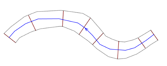
The results are mapped only within the extent of cross sections as illustrated in Figure 15.1.

Figure 15.1        Illustration of area covered by the 2D map based on cross sections extent. Blue line represents the river branch, brown lines represent cross sections and the dashed black lines represent the area where results will be mapped.

No calculation of results will take place outside the cross sections extent, and the maps obtained, will therefore represent exactly what the model calculates during the actual simulation.

An example of a flood map produced through the map-feature is presented in Figure 15.2:

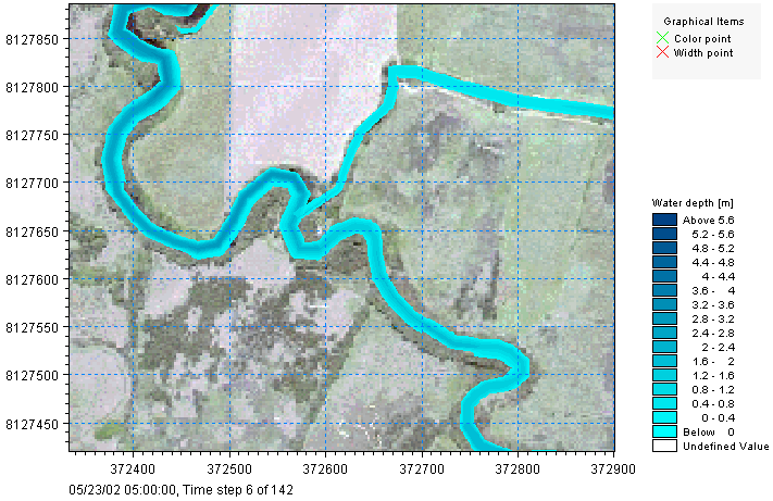
Figure 15.2        An example of a 2D flood inundation map presented in the Result Viewer

For each created map, the following parameters and options must be speci­fied.

Name

The identification name of the map output.

File name

The path and the name of the dfs2 file storing the map results.

Item

The item being mapped in the result file. Only one item can be mapped in each file. Various results items may be mapped.

The complete list consists of:

-          –         Water level: this option creates a map of water level. The water level is assumed to be constant along the cross sections, and is then interpolated in the longitudinal direction.

-          –         Water depth: this option creates a map of water depth, being the dif­ference between the above water level and the interpolated bed level.

-          –         Velocity: with this option, the velocity is recomputed based on the water depth in each cell of the grid.

-          –         Velocity * depth: this provides a derived result computed as velocity times depth

-          –         Advection-Dispersion component: this option creates a map of the concentration of the selected component.

-          –         DEM: this option generates a digital elevation model (DEM) for the river bed, based on the topography from the cross sections and the river branches. With this option, no period needs to be specified.

-          –         (h, p, q): this option produces a file containing the three items Water depth, P-flux and Q-flux. This map type is primarily relevant for MIKE FLOOD simulations (coupled 2D- and 1D-simulations), as the map file can be burnt afterwards in the 2D result file in order to get a combined map, with the same result items on both the 1D and 2D domain.

Please refer to the MIKE 1D reference manual for details about the mapping procedure.

Type

The maps may be of three types:

-          –         Maximum: the overall maximum value throughout the simulation period for each cell included in the map.

-          –         Minimum: the overall minimum value throughout the simulation period for each cell included in the map.

-          –         Dynamic: time-varying map able to animate the results.

Component

The selected Advection-Dispersion component to be mapped, when the selected Item is 'AD result'.

Cell size

The cell size of the dfs2 output file. The cell size controls the spatial resolu­tion of the map.

Rotation

The rotation of the dfs2 output file. The rotation is defined as the angle between true north and the y-axis of the grid, measured clockwise. When a rotation is applied, the grid is rotated from its lower left corner, i.e. this corner remains at the same coordinates whereas the three other corners are moved.

Extent def.

This controls the way the extent of the map in the two spatial dimensions is defined. Two options are available:

-          –         Lengths: with this option, you specify the width and height of the rec­tangle to define the dimensions along the two horizontal axes. MIKE HYDRO will derive the extent of the map from the origo and these lengths.

-          –         No. of cells: with this option, you specify the number of cells of the grid in the two spatial dimensions, J being the number of cells east­ward and K being the number of cells northward.

X0

The X coordinate of the lower left corner of the grid.

Y0

The Y coordinate of the lower left corner of the grid.

Width

The length of the grid in the eastward direction. This field can be edited only when the extent is defined using the option 'Lengths'. When the extent is defined using the option 'No. of cells', the field displays the width which is automatically derived from the number of J cells and the cell size.

Height

The length of the grid in the northward direction. This field can be edited only when the extent is defined using the option 'Lengths'. When the extent is defined using the option 'No. of cells', the field displays the height which is automatically derived from the number of K cells and the cell size.

No. of J cells

Number of cells of the grid in the eastward direction (note that this dimension is not strictly from West to East when the rotation is different than 0). This field can be edited only when the extent is defined using the option 'No. of cells'. When the extent is defined using the option 'Lengths', the field displays the number of cells which is automatically derived from the width and the cell size.

No. of K cells

Number of cells of the grid in the northward direction (note that this dimension is not strictly from South to North when the rotation is different than 0). This field can be edited only when the extent is defined using the option 'No. of cells'. When the extent is defined using the option 'Lengths', the field displays the number of cells which is automatically derived from the height and the cell size.

Storing frequency

The storing frequency controls the interval between two time steps saved in the output file. The unit used for the specified value is selected under 'Storing unit'. This parameter is only available for the 'Dynamic' type of map.

Storing unit

The unit in which the storing frequency is expressed. This parameter is only available for the 'Dynamic' type of map.

Period

This parameter controls how the period, for which the map is produced, is defined. Two options are available:

-          –         Simulation period: with this option, the results are mapped for the full simulation period, as defined under the 'Simulation period' menu.

-          –         Selected period: with this option, the results are mapped for a limited period specified manually. This option may be used in order to reduce the weight of the output file.

This parameter is only available for the 'Dynamic' type of map. When the type is either 'Minimum' or 'Maximum', the period is always the simulation period.

Start

The date and time starting from which the results are mapped. This date and time cannot be prior to the start date of the simulation.

End

The date and time at which the results stop to be mapped. This date and time cannot be posterior to the end date of the simulation.

Note: The extent of the map may be graphically defined by clicking 'Draw rec­tangle on the map' and dragging a rectangle on the map. This button is active only when the rotation is different than 0. Once defined, the rectangle may be edited (and edits must be saved) but it cannot be deleted.