River module examples

This section includes a brief overview of the River Modules examples included in the MIKE HYDRO Installation.

Demo
Vida
Dambreak
Data Assimilation

Demo

The enclosed Demo example comes from a setup of Cali River which has been modified to reduce the original number of input elements (cross-sec­tions and river branches) to keep within the limitations of MIKE HYDRO Demo version.

The setup comprises 3 branches and 10 cross-sections. The boundaries con­sist of a single recorded upstream inflow and two downstream water levels conditions.

Using the predefined settings for input files, the simulation period and time step, it is possible to perform a simulation and view the results.

Vida

This example is a setup from a stream (small river) in Denmark, named ‘Vid-Å’. The setup was developed by DHI for a project conducted in 1997.

The Vida setup comprises a main river branch with several smaller tributaries feeding into the main river. Boundary conditions are defined as inflow hydro­graphs on all upstream boundaries and a downstream tidal boundary at the sea. The downstream boundary is defined by applying measured water levels covering a large number of tidal periods.

All input files required to perform the hydrodynamic computation are present.

Dambreak

This example describes a dam failure on a short stretch of a river, and simu­lates the subsequent flood wave.

The model comprises a 12 kilometers-long river including 6 cross-sections, with a mean slope of 0.064% and a reservoir with a volume of 0.3 million m³.

The boundary conditions set for this model are:

·         Upstream boundary condition: time varying discharge with a total dura­tion of 24 hours, a peak time of 11 hours and a peak discharge of 30 m3/s.

·         Downstream boundary condition: free outflow.

The initial water level in the reservoir is set at 111 m.

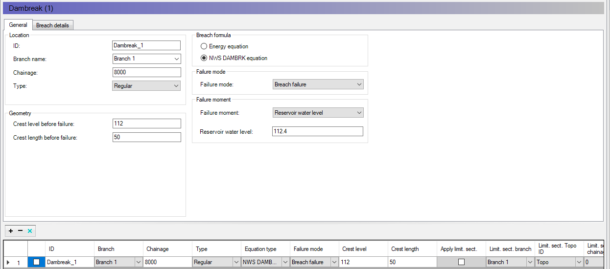
The dambreak structure is defined with the following settings:

·         Crest level before failure: 112 m

·         Crest length before failure: 50 m

·         Failure mode = Breach failure

·         Failure moment = Reservoir water level

·         Reservoir water level = 112.4 m.

Figure 2.5           Dambreak example

The dam simulated with these settings has a crest level of 112 m and a crest length of 50 m before the failure, and the failure will be triggered when the water level in the reservoir reaches 112.4 m, i.e. when the dam crest is over­topped by 0.4 m. The failing mechanism is a breach failure, which means that the breach develops starting from the dam crest and enlarges over time.

The variation of the breach geometry (after the time of failure) is defined by a series of varying parameters in the 'Breach details' tab: breach bottom level, breach width and breach slope. The breach detail time series contains the data shown in the table below.

Until the water level in the reservoir has reached the critical level of 112.4 m, the dam is represented by a weir with the specified crest level and width before failure. When the water level reaches this critical level, the trapezoidal breach develops with the geometry defined in the time series, in this example with a progressive change starting from a width of 0 m at level 112 m. After 10 minutes, the breach has reached its final dimensions, which can be seen on the picture below.

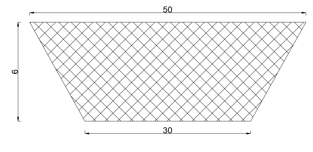
Figure 2.6           Final breach geometry

After running the simulation, it is possible to observe how the hydrograph near the dam is affected by the failure.

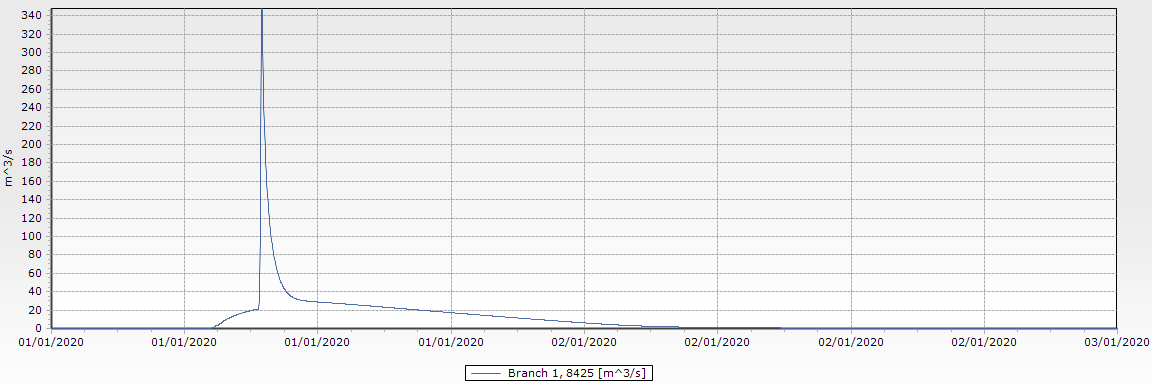
Figure 2.7           Flood wave generated by the breach in the dam

Data Assimilation

This example shows how an automatic correction can be applied to the simu­lation in order for the results to match observed data, in a real-time applica­tion (forecasting flow conditions after the last time with observed data).

The model comprises a 12 kilometers-long river including 6 cross-sections, with a mean slope of 0.064%.

The boundary conditions set for this model are:

·         Upstream boundary condition: time varying discharge with a total dura­tion of 24 hours, a peak time of 11 hours and a peak discharge of 30 m³/s.

·         Downstream boundary condition: free outflow.

The Data Assimilation module is set up with the following settings:

·         Mode: Updating with weighting function

·         First updating time step = 0

·         Time of forecast = 2020-01-02 00:00:00

The correction will therefore be applied to the river with a weighting function, from the first time step of the simulation up until the time of forecast.

There is only one measurement location where the model will be updated, at chainage 8200 m. The observed water level is supplied in the time series file Observed_water_level.dfs0. The correction, which must be applied so that the simulated water level at chainage 8200 m matches the observed level, is uniformly (constant type) distributed from chainage 7800 to 8200 m.

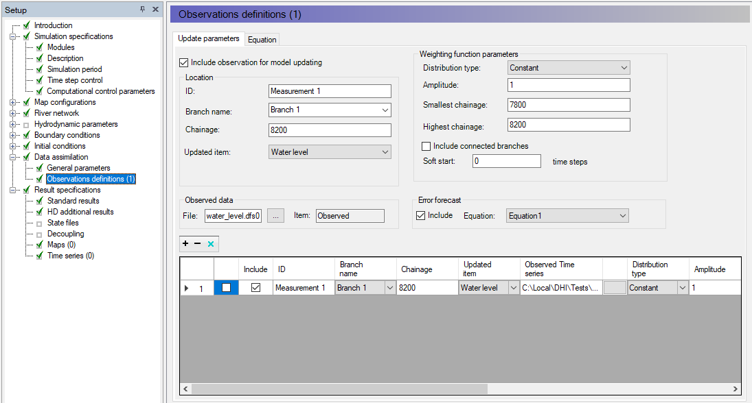
Figure 2.8           Update parameters page

After the time of forecast, the model can no longer be updated on observed data. To avoid rapid changes due to the correction being suddenly stopped, the 'Error forecast' option is included: in this case the correction calculated before the time of forecast is extrapolated in the forecast period, using the equation specified in the 'Equation' tab.

The equation is defined as 0.999* E(-1) in this example, where E(-1) is the error from the previous time step. The correction will therefore progressively decrease over time.

After running the simulation, it is possible to verify that the simulated water level at chainage 8200 m matches the observed water level up until the time of forecast. After that time, the simulated water level progressively converges towards the water level which would be calculated without data assimilation. This can be verified by comparing results with and without data assimilation with the observed data, as shown below.

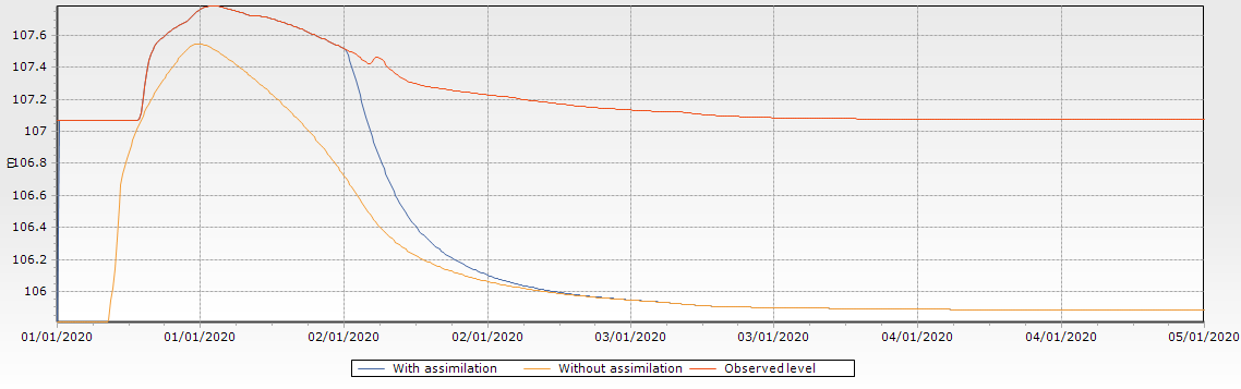
Figure 2.9           Effect of data assimilation on the simulated water level