
NAM
The NAM model is a deterministic, lumped and conceptual rainfall-runoff model accounting for the water content in up to four different storages. NAM can be prepared in a number of different modes depending on the requirement. As default, NAM is prepared with nine parameters representing the surface zone, root zone and the groundwater storages.
In addition, NAM contains provision for:
· Extended description of the groundwater component.
· Two different degree day approaches for snow melt.
The NAM Rainfall-runoff component is accessed once the NAM model is selected under the General tab.
More details on the NAM model can be found in the ‘MIKE 1D Reference’ manual.
In the NAM model, the following sections can be found:
The parameters of each section are specified for each representative catchment.
The NAM Rainfall-runoff simulation covers the period as specified in the Simulation period dialogue (“Simulation Period” on page 52).
· Maximum water content in surface storage (Umax). It represents the cumulative total water content of the interception storage (on vegetation), surface depression storage and storage in the uppermost layers (a few cm) of the soil. Typical values are between 10-20 mm.
· Maximum water content in root zone storage (Lmax). It represents the maximum soil moisture content in the root zone, which is available for transpiration by vegetation. Typical values are between 50-300 mm.
· Overland flow runoff coefficient (CQOF). It determines the division of excess rainfall between overland flow and infiltration. Values range between 0.0 and 1.0
· Time constant for routing interflow (CKIF). It determines the amount of interflow, which decreases with larger time constants. Values in the range of 500-1000 hours are common.
· Time constants for routing overland flow (CK1, CK2). They determine the shape of hydrograph peaks. The routing takes place through two linear reservoirs (serially connected) with different time constants, expressed in [hours]. High, sharp peaks are simulated with small time constants, whereas low peaks, at a later time, are simulated with large values of these parameters. Values in the range of 3-48 hours are common.
· Root zone threshold value for overland flow (TOF). It determines the relative value of the moisture content in the root zone (L/Lmax) above which overland flow is generated. The main impact of TOF is seen at the beginning of a wet season, where an increase of the parameter value will delay the start of runoff as overland flow. Threshold value range between 0 and 70% of Lmax, and the maximum value allowed is 0.99.
· Root zone threshold value for interflow (TIF). It determines the relative value of the moisture content in the root zone (L/Lmax) above which interflow is generated.
For most NAM applications only the Time constant for routing baseflow (CKBF) and possibly the Root zone threshold value for groundwater recharge (TG) need to be specified and calibrated. However, to cover also a range of special cases, such as groundwater storages influenced by river level variations, a number of additional parameters can be modified.
The groundwater parameters are:
· Root zone threshold value for GW recharge (TG). It determines the relative value of the moisture content in the root zone (L/Lmax) above which groundwater (GW) recharge is generated. The main impact of increasing TG is less recharge to the groundwater storage. Threshold values range between 0 and 70% of Lmax and the maximum value allowed is 0.99.
· Time constant for routing baseflow (CKBF). It can be determined from the hydrograph recession in dry periods. In rare cases, the shape of the measured recession changes to a slower recession after some time. To simulate this, a second groundwater reservoir may be included, see the extended components below.
· Ratio of GW-area to catchment area (Carea). This parameter describes the ratio of the groundwater catchment area to the topographical surface water catchment area, which is specified under the General tab. Local geological condition may cause part of the infiltrating water to drain to another catchment. This loss of water is described by a Carea less than one. Usual value: 1.0.
· Specific yield of groundwater reservoir (Sy). This parameter should be kept at the default value except for the special cases in which the groundwater level is used for NAM calibration. This may be required in riparian areas, for example, where the outflow of groundwater strongly influences the seasonal variation of the levels in the surrounding rivers. Simulation of groundwater level variation requires values of the specific yield Sy and of the groundwater outflow level GWLBFO, which may vary in time. The value of Sy depends on the soil type and may often be assessed from hydro-geological data, e.g. test pumping. Typically values of 0.01-0.10 for clay and 0.10-0.30 for sand are used.
· Maximum GW-depth causing baseflow (GWLBF0). It represents the distance in meters between the average catchment surface level and the minimum water level in the river. This parameter should be kept at the default value except for the special cases in which the groundwater level is used for NAM calibration, cf. Sy above.
· Seasonal variation of GW-depth causing baseflow. In low-lying catchments the annual variation of the maximum groundwater depth may be of importance. This variation relative to the difference between the maximum and minimum groundwater depth can be entered if the checkbox is ticked. The monthly values are given relative to the difference between GWLBF0 and GWLBF_min [0-1]. This is done in the Seasonal variation page, in the column Variation of groundwater maximum water depth.
· Minimum GW-depth for seasonal variation (GWLBF_min). If the Seasonal variation of GW-depth causing baseflow is selected, the minimum GW-depth level [m] has also to be entered for the calculations.
· Capillary flux, depth for unit flux (GWLBF1). It is defined as the depth of the groundwater table generating an upward capillary flux of 1 mm/day when the upper soil layers are dry corresponding to wilting point. The effect of capillary flux is negligible for most NAM applications. Keep the default value of 0.0 to disregard capillary flux.
· Use abstraction. If this option is selected, it is possible to specify the groundwater abstraction depth from the catchment.
The input type of this variable can be:
– Time series. If this option is selected, a time series of abstraction depth has to be entered in the Time series page.
– Seasonal variation. This option allows to specify monthly values of abstraction depth in the Seasonal variation page.
· Use lower baseflow, recharge to groundwater (Cqlow). The groundwater recession is sometimes best described using two linear reservoirs, with the lower usually having a larger time constant. In such cases, the recharge to the lower groundwater is specified here as a percentage of the total recharge.
· Time constant for routing lower baseflow (Cklow). It is specified for Cqlow > 0 as a baseflow time constant, which is usually larger than the CKBF.
The snow module simulates the accumulation and melting of snow in a NAM catchment. It is included in the model when the ‘Include snow melt’ checkbox is ticked.
Two degree day approaches can be applied: a simple lumped calculation or a more advanced distributed approach. The simple degree-day approach uses only two overall parameters: a Constant Degree day coefficient and a Base temperature (snow/rain). The distributed approach allows the user to specify a number of elevation zones within a catchment with separate snow melt parameters, temperature and precipitation input for each zone.
The snow melt module uses a temperature input time series, usually mean daily temperature. This has to be specified in the Time series tab.
The snow melt parameters are:
· Constant Degree day coefficient (Csnow). The content of the snow storage melts at a rate defined by the degree-day coefficient multiplied by the temperature difference above the Base temperature. Typical values for Csnow are 2-4 mm/day/C.
· Base temperature (snow/rain) (To). The precipitation is retained in the snow storage only if the temperature is below the base temperature, whereas it is by-passed to the surface storage (U) in situations with higher temperatures. The base temperature is usually at or near zero degree C.
It is also possible to specify other input parameters for the snow melt module, if the relative checkboxes are ticked. These are:
· Variation of degree day coefficient. This option is selected when the melting coefficient is varying in time, instead of being constant. The input for this model can be specified in two ways:
– Specify as time series file. In this case the melting coefficient is specified in a time series that has to be loaded in the Time series section.
– Specify as seasonal variation. If this option is selected, monthly values of the degree day coefficient for snow melt must be specified in the Seasonal variation section.
· Radiation coefficient (Radiation file on time series page). This option may be introduced when time series data for incoming radiation is available. The time series input file is specified separately on the Time series section. The total snow melt is calculated as a contribution from the traditional snow melt approach based on Csnow (representing the convective term) plus a term based on the radiation.
· Rainfall degree day coefficient. This option may be introduced when the melting effect from the advective heat transferred to the snow pack by rainfall is significant. This effect is represented in the snow module as a linear function of the precipitation multiplied by the rainfall degree coefficient and the temperature deviation above the base temperature.
The Elevation zones tab becomes available when snow melt is included in the model. When the ‘Delineate catchment into elevation zones for snow modelling’ option is selected, the snow melt distributed approach is applied. Following this approach, the catchment is divided into a certain number of elevation zones, each with specific snow melt parameters, temperature and precipitation inputs.
The general parameters that have to be specified for the snow melt model are:
· Number of elevation zones
· Reference level for temperature station. This parameter defines the altitude [m] of the reference temperature station. This station is used as a reference for calculating the temperature and precipitation within each elevation zone (the file with temperature data is specified on the Time series page).
· Dry temperature lapse rate. It specifies the vertical gradient [C/100 m] for adjustment of temperature under dry conditions. The temperature in the actual elevation zone is calculated based on a linear transformation of the temperature from the reference station to the actual zone, the correction being defined as the dry temperature lapse rate multiplied by the difference in elevations between the reference station and the actual zone.
· Wet temperature lapse rate. This parameter specifies the vertical gradient [C/100 m] for adjustment of temperature under wet conditions defined as days with precipitation higher than 10 [mm]. The temperature in the actual elevation zone is calculated based on a linear transformation of the temperature from the reference station to the actual zone, the correction being defined as the wet temperature lapse rate multiplied by the difference in elevations between the reference station and the actual zone.
· Reference level for precipitation station. This parameter defines the altitude, expressed in [m], at the reference precipitation station (the file with precipitation data is specified on the Time series page).
· Correction of precipitation rate. This parameter specifies the vertical gradient for adjustment of precipitation and is expressed in [percent/100 m]. The precipitation in the actual elevation zone is calculated based on a linear transformation of the precipitation from the reference station to the actual zone, the correction being defined as correction of precipitation rate [percent/100 m] multiplied by the difference in elevation between the reference station and the actual zone.
The specific parameters for each elevation zone are entered in the table at the bottom of the page. These are:
· Zone. Zone number ID automatically assigned by the programme.
· Elevation. The elevation of each zone is specified in the table as the average elevation of the zone. The elevation must increase from zone (i) to zone (i+1).
· Area. The area of each zone is specified in the table. The total area of the elevation zones must equal the area of the catchment.
· Min storage for full coverage. This parameter defines the required amount of snow to ensure that the zone area is fully covered with snow. When the water equivalent of the snow pack falls under this value, the area coverage (and the snow melt) will be reduced linearly with the snow storage in the zone.
· Max storage in zone. This value defines the upper limit for snow storage in a zone. Snow above this value will be automatically redistributed to the neighbouring lower zone.
· Max water retained in snow. It defines the maximum water content in the snow pack of the zone. Generated snow melt is retained in the snow storage as liquid water until the total amount of liquid water exceeds this water retention capacity. When the air temperature is below the base temperature To, the liquid water of the snow re-freezes with rate Csnow.
· Dry temperature correction. The actual temperature correction for dry conditions to estimate actual temperature for the specific zone.
· Wet temperature correction. The actual temperature correction for wet conditions to estimate actual temperature for the specific zone.
· Precipitation correction. The relative correction for precipitation, expressed in percent, to estimate the precipitation for the specific zone.
The ‘Calculate’ button above the table fills the three columns in the table for Dry temperature correction, Wet temperature correction and Precipitation correction, based on the specified rates above.
An irrigation module is included in the rainfall-runoff model when the ‘Include irrigation’ box is ticked. This irrigation module has a different function than the one defined for the irrigation water user. While the latter is used to calculate water balances at the catchment scale, the irrigation module in the rainfall-runoff model is only used for adjusting the water balance in the NAM model. The purpose of the NAM irrigation module is that of simulating the runoff and groundwater recharge/baseflow from the irrigated areas, so that NAM can be calibrated for the non-irrigated part of the catchment.
Minor irrigation schemes within a catchment will normally have negligible influence on the catchment hydrology, unless transfer of water over catchment boundaries is involved. Large schemes, however, may significantly affect the runoff and the groundwater recharge through local increases in evapotranspiration and infiltration as well as through operational and field losses.
The irrigation module of NAM may be applied to describe the effect of irrigation on the following aspects:
· The overall water balance of the catchment. This will be affected mainly by the increased evapotranspiration and by possible external water sources for irrigation.
· Local infiltration and groundwater recharge in irrigated areas.
· The distribution of catchment runoff amongst different runoff components (overland flow, interflow, baseflow). This may be influenced by the increased infiltration in irrigated areas as well as by local abstraction of irrigation water from groundwater or streams.
The irrigation parameter is:
· Infiltration rate at field capacity (K0-inf). This parameter defines the rate of infiltration at field capacity [mm/h].
The Irrigation sources in percent are:
· Local groundwater (PC_LGW). Percentage of water for irrigation supplied by groundwater sources.
· Local river (PC_LR). Percentage of water used for irrigation supplied by a local river.
· External river (PC_EXR). Percentage of water for irrigation supplied by a river external from the catchment defined in NAM.
Another irrigation option is:
· Include crop coefficients and operational losses. If this checkbox is ticked, additional irrigation module parameters can be specified as monthly values in the Seasonal variation page.
These are:
– Irrigation crop coefficient. This parameter, also defined as Kc, allows to quantify the amount of water required (and transpired) by the crop. Different crops have different crop coefficient. Kc is multiplied by the reference ET of a standard crop (grass) to calculate the water demand of the crop of interest.
– Irrigation operational and conveyance losses in percent of abstract water. These represent the system losses of irrigation water for the different components/processes:
Groundwater
Overland flow
Evaporation
The initial relative water contents of surface and root zone storage must be specified as well as the initial values of overland flow and interflow. Initial values for baseflow must always be specified. When lower baseflow is included, a value for the initial lower baseflow must also be specified.
Initials values of the snow storage are specified when the snow melt routine is used. When the catchments are delineated into elevation zones, the snow storage and the water content in each elevation zone are specified.
The parameters of the different subsections are:
· Relative water content in surface storage [0, 1] (U/UMax). This value ranges between zero and one, where one indicates wet initial conditions and zero dry initial conditions.
· Relative water content in root zone storage [0, 1] (L/LMax). This value ranges between zero and one.
· Overland flow (QOF). The overland flow at the beginning of the simulation, which is normally estimated from the hydrograph [m3 s-1].
· Interflow (QIF). The interflow at the beginning of the simulation, which is normally based estimated from the hydrograph [m3 s-1].
· Baseflow (BF). The baseflow at the beginning of the simulation, which is normally estimated from the hydrograph [m3 s-1].
· Lower baseflow (BF - low). The lower baseflow at the beginning of the simulation, which is normally estimated from the hydrograph
[m3 s-1].
If the Elevation zones option is not selected:
· Global value. This parameter represents the actual initial snow storage in [mm] over the entire catchment.
If the Elevation zones option is selected:
· Zone, Snow storage, and Water in snow. If the snow model is defined using elevation zones, it is required to enter for each zone the initial Snow storage in [mm] and the Water in snow, also in [mm], defining the water content in the snow pack.
It is possible to use an automatic optimisation procedure to calibrate the 12 most important parameters in the NAM model. The calibration routine used in NAM is based on a multi-objective optimisation strategy, the SCE algorithm. The procedure implemented in NAM allows to simultaneously optimise four different calibration objectives or a combination of them. A description of the SCE algorithm is given in the ‘Autocal User Guide’.
To include the Autocalibration routine in NAM, tick the ‘Include autocalibration’ checkbox.
Calibration parameters
The parameters which can be included in the autocalibration routine are listed in the Calibration parameters table:
· Maximum water content in surface storage (Umax).
· Maximum water content in root zone storage (Lmax)
· Overland flow runoff coefficient (CQOF)
· Time constant for interflow (CKIF)
· Time constant 1 for routing overland flow (CK1)
· Time constant 2 for routing overland flow (CK2)
· Root zone threshold value for overland flow (TOF)
· Root zone threshold value for interflow (TIF)
· Root zone threshold value for groundwater recharge (TG)
· Time constant for routing baseflow (CKBF)
· Lower baseflow, recharge to lower reservoir (Cqlow)
· Time constant for routing lower baseflow (Cklow).
If the ‘Fit’ checkbox is ticked, the parameter is included in the autocalibration. The table also contains the following columns:
· Initial value. It is the value for the parameter specified in the Surface-rootzone or Groundwater page and used in the first model simulation.
· Lower Bound and Upper Bound are the minimum and maximum values that the parameter can assume and therefore define its range of variation.
Objective functions
In automatic calibration, the calibration objectives have to be formulated as numerical goodness-of-fit measures that are optimised.
Four calibration objectives are defined as numerical performance measures in the Autocalibration routine of NAM. These are selected and used by ticking the relative checkboxes.
· Overall water balance. This defines the agreement between the average simulated and observed catchment runoff overall volume error.
· Overall root mean squared error. This measure defines the overall agreement of the shape of the simulated hydrograph with the observed one.
· Peak flow RMSE. This optimisation measure defines the agreement of simulated and observed peak flows events. If this measure is selected, the minimum river discharge value above which the flow is defined as peak flow has to be specified in the Peak flow field.
· Low flow RMSE. This optimisation measure defines the agreement of simulated and observed low flows events. If this measure is selected, the maximum river discharge value below which the flow is defined as low flow has to be specified in the Low flow field.
Other input parameters are:
· Maximum number of evaluations. Here one of the stopping criteria of the auto calibration routine is specified. The automatic calibration will stop either when the optimisation algorithm ceases to give an improvement in the calibration objective or when the maximum number of model evaluations is reached.
· Initial number of day excluded. This is a warm up period that will be disregarded when calculating the objecting function.
Running the autocalibration
After having entered the autocalibration parameters, the autocalibration procedure starts when launching a normal simulation. When the optimisation routine is completed, the list of the parameters generated during the optimisation and the relative objective functions are made available in the CatchmentName-Autocal.txt file. If the Calibration plot option has been selected in the General tab, a CatchmentName.plc file is also produced. This file shows the differences between the observed and the best simulated runoff data, and can be opened in the Plot Composer.
Note: The various NAM parameters shown in the Rainfall-runoff tab will not be automatically updated with the optimal parameter set. To visualize the optimized parameters, either close (without saving) the MIKE HYDRO file and re-open it, or check the created text file CatchmentName-Autocal.txt.
In this section it is possible to enter the values of some selected time varying parameters. Monthly values have to be assigned to the parameters. Whether a parameter has a constant or a seasonal varying value is determined in the different sections of the NAM model.
It is possible to specify a seasonal variation for the parameters:
· Variation of groundwater maximum water depth. Seasonal variation of GW-depth causing baseflow. From Groundwater tab.
· Abstraction. Groundwater abstraction depth. From Groundwater tab.
· Degree day coefficient for snow melt. Melting coefficient for snow melt. From Snow melt tab.
· Irrigation crop coefficient. Parameter to quantify the amount of water required (and transpired) by the crop. From Irrigation tab.
· Irrigation operational and conveyance losses in percent of abstracted water. System losses of irrigation water for the different components/processes: Groundwater, Overland flow and Evaporation. From Irrigation tab.
In this section the input time series of the rainfall-runoff model are entered. Depending on which module of the model is used, these are:
· Rainfall. Always to be entered. A time series, representing the average catchment rainfall. The time interval between values may vary through the input series. The rainfall specified at a given time should be the rainfall volume accumulated since the previous value.
· Evaporation. Always to be entered. The potential evaporation is typically given as monthly values. Like rainfall, the time for each potential evaporation value should be the accumulated volume at the end of the period it represents. The monthly potential evaporation in June should be dated 30 June or 1 July.
· Observed discharge. This time series has to be entered if the Autocalibration module is used or the ‘Calibration plot’ option has been selected in the General tab. The inclusion of the observed discharge will automatically enable additional outputs which include a calibration plot with comparison of observed and simulated discharge and calculation of statistical values.
· Temperature. A time series of temperature, usually mean daily values, is required only if snow melt calculations are included in the simulations.
· Irrigation. To be entered when the irrigation module of the rainfall-runoff module is included.
· Abstraction depth. To be entered when the ‘Use abstraction’ option in the Groundwater tab is selected and ‘Time series file’ is specified.
· Radiation. To be entered when the ‘Radiation coefficient’ option in the Snow melt tab is selected.
· Degree day coefficient. To be entered when the ‘Variation of degree day coefficient’ option in the Snow melt tab is selected.
Weighted time series may be used for some time series by enabling ‘Use weighted time series’. This adds a new tab ‘TS weighted rainfall/evaporation/temperature’ to the window (see below).
To use weighted time series, ‘Use weighted time series’ must be enabled under the Time series tab - see above. Under the TS weighted tab the following may be defined:
Allow gap in time series
If ‘Allow gap in time series’ is enabled, simulation will proceed despite missing data (gap) in the time series. If ‘Allow gap in time series’ is disabled, simulation will terminate with an error message if missing data (gaps) are encountered in the time series.
Distribution in time
If data is available from stations reporting at different frequencies, e.g. both daily and hourly stations, the Distribution in time of the average catchment rainfall may be determined using a weighted average of the high-frequency stations. You may, for example, use all daily and hourly stations to determine the daily mean rainfall over the catchment and subsequently use the hourly stations to distribute (desegregate) this daily rainfall in time.
Weighted average combinations
To specify a weighted average combination, add time series by clicking the Append ‘+’ button above the table to add a new row, then click the browse ‘...’ button to select a time series or create a new file and enter the weight to be assigned to that time series. Repeat the steps for all relevant time series/stations.
The weighted average values Tweighted are computed using the following formula:
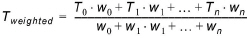
where Tn is the value from time series n and wn the corresponding weight.
If data are missing from one or more time series/stations, and ‘Allow gap in time series’ is enabled, the Mean Area Weighting algorithm will ignore the time series with missing data.
In the present version it is possible to specify only one weighted average combination.
![]()