Governing Equations

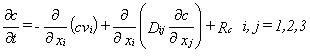
The transport of solutes in the saturated zone is governed by the advection-dispersion equation, which for a porous medium with uniform porosity is

(33.3)   

where c is the concentration of the solute, Rc is the sum of the sources and sinks, D_ij is the dispersion coefficient tensor and v_i is the velocity tensor.

The advective transport is determined by the water fluxes (Darcy velocities) calculated during a MIKE SHE WM simulation. To determine the groundwater velocity, the Darcy velocity is divided by the effective porosity

(33.4)   

where q_i is the Darcy velocity vector and q is the effective porosity of the medium.

The mathematical formulation of the dispersion of the solutes follows the tra­ditional formulations generalised to three dimensions. This formula was developed assuming that the dispersion coefficient is a linear function of the mean velocity of the solutes. In the three-dimensional case of arbitrary flow-direction in an anisotropic aquifer, the dispersion tensor, D_ij, contains nine elements, giving a total of 36 dispersivities. The general formulation of the dispersion tensor is derived in Scheidegger (1961) and can be written as

(33.5)   

where a_ijmn is the dispersivity of the porous medium (a fourth order tensor), v_n and v_m are the velocity components, and U is the magnitude of the velocity vector.

The derivation of D_ij and a_ijmn in MIKE SHE follows the work of Bear and Ver­ruijt (1987). Two simplifications have been introduced with respect to disper­sivity

·         isotropy, and

·         anisotropy with axial symmetry around the z-axis.

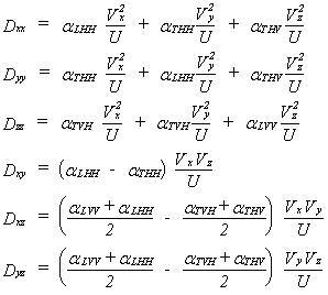
These simplifications are reflected in the number of non-zero dispersivities to be specified. Under isotropic conditions the dispersivity tensor, a_ijmn, solely depends on the longitudinal dispersivity, a_L, and the transversal dispersivity, a_T, in the following manner:

(33.6)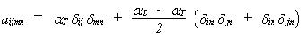   

where d_ij is the Kronecker delta (with d_ij=0 for i¹j and dij=1 for i=j). In the Car­tesian co-ordinate system applied in MIKE SHE, the velocity components in the coordinate directions are denoted V_x, V_y and V_z. Thus, we obtain the fol­lowing expressions for the dispersion coefficients:

(33.7)   

This is the general equation for the dispersion coefficients in an isotropic medium for an arbitrary mean flow direction. If the mean flow direction coin­cides with one of the axis of the Cartesian coordinate system the expression for the dispersion coefficients simplifies even further (e.g. if V_y and V_z are equal to zero then D_xy, D_xz and D_yz will also be zero).

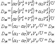
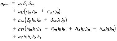
Under fully anisotropic conditions, the dispersion coefficients depend on 36 dispersivities which is impractical to handle and estimate in practice. Thus, if we assume that the porous medium is symmetric around one of the axis, the number of non-zero dispersivities can be limited to five. This assumption is true if the medium is made up of layers normal to the axis of symmetry, which is the case for some geological deposits. Under these conditions the following expression for the a_ijmn terms (Bear and Verruijt (1987)) have been derived:

(33.8)   

where a_I, a_II, a_III, a_IV and a_V are independent parameters and h is a unit vector directed along the axis of symmetry. In MIKE SHE AD it is assumed that the axis of symmetry always coincides with the z-axis and h becomes equal to (0,0,1). Five dispersivities are then introduced

–         a_LHH -    the longitudinal dispersivity in the horizontal direction for hori­zontal flow

–         a_THH -    the transversal dispersivity in the horizontal direction for hori­zontal flow

–         a_LVV -    the longitudinal dispersivity in the vertical direction for vertical flow

–         a_TVH -    the transversal dispersivity in the vertical direction for horizon­tal flow

–         a_THV -    the transversal dispersivity in the horizontal direction for verti­cal flow

Thus, the dispersion coefficients can be written explicitly by combining Eq. (33.5) and Eq. (33.8) as follows:

(33.9)   

and for symmetrical reasons D_xy = D_yx, D_xz = D_zx and D_yz = D_zy.

Note that Eq. (33.9) can simplify to Eq. (33.7) if a_LHH=a_LVV=a_L and  a_THH=a_TVH=a_THV=a_T 

Burnett and Frind /11/ suggest that the dispersion should at least allow for the use of two transverse dispersivities - a horizontal transverse dispersivity and a vertical transverse dispersivity - to describe the difference in transverse spreading which is greater in the horizontal plane than in the vertical plane. In comparison, MIKE SHE uses all five dispersivities.

The determination of the five dispersivities is always difficult so often one has to rely on experience or on empirically derived values.

The dispersion term in the advection-dispersion equation accounts for the spreading of solutes that is not accounted for by the simulated mean flow velocities (the advection). Therefore, it is obvious that the more accurate you describe the spatial variability in the hydrogeologic regime and if the grid is sufficiently fine (i.e. the variations in the advective velocity) the smaller the dispersivities you need to apply in the model. Recent laboratory and field research have shown a relationship between the spatial variability of hydro­geologic parameters and the dispersivities. However, it is still difficult to obtain sufficient knowledge about the spatial variability of, for example the hydraulic conductivity, to determine macro dispersivities applicable for solute transport models.