Solution Scheme

Regular Grid

The numerical solution to the advection-dispersion equation in MIKE SHE AD is based on the QUICKEST method. Leonard /38/ originally introduced this method, which was further developed by Vested et. al. /53/. It is a fully explicit scheme, which applies upstream differencing for the advection term and cen­tral differencing for the dispersion term. The equations are developed to third order and the scheme is mass conservative.

When the vertical discretisation is defined in a regular grid with uniform thick­ness of all layers except the upper and the lower ones the numerical scheme follows the fully three-dimensional formulation below.

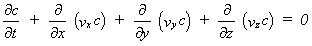
Neglecting the dispersion terms and the source/sink term and assuming that the flow field satisfies the equation of continuity and varies uniformly within a grid cell the advection-dispersion equation may be written in mass conserva­tion form as:

(33.10)   

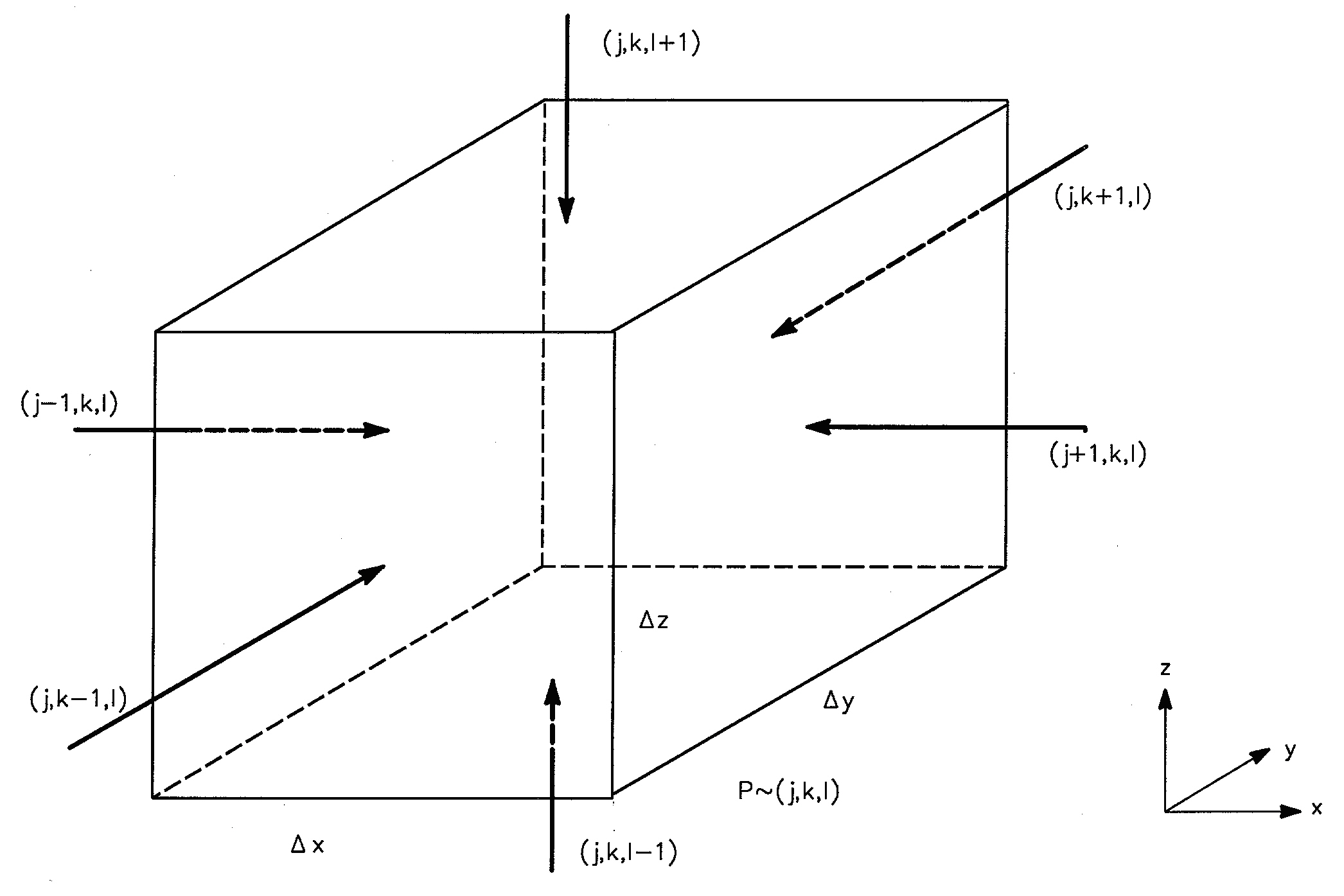
Figure 33.3        Control volume defining an internal SZ grid.

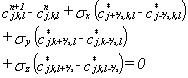
For the control volume shown in Figure 33.3 this equation is written in finite difference form as:

(33.11)   

where n denotes the time index.

In Eq. (33.11) s_x, s_y and s_z are the directional Courant numbers defined by

(33.12)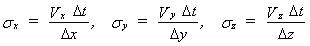   

and the c*-terms are the concentrations at the surface of the control volume at time n. As these terms are not located at nodal points they have to be inter­polated from known concentration values:

(33.13)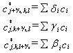   

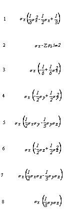
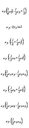
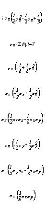
The concentration c_i is the concentration around the actual point, for example (j-1,k-1,l) and the weights d_i, g_i and b_i are determined in such a way that the scheme becomes third-order accurate. The determination of the weights is demonstrated in Vested et al. (1992) and their values are listed in Table 33.2.

A number of 8 weights has proven to be an adequate choice and their loca­tion for the determination of the c*_j+½,k,l is shown in Figure 33.4. The other “boundary” concentrations are found in a similar way

.

Table 33.2          Weight functions for advective transport

Li	Ki	Ji

The locations of the weights are determined by the points that enter into the discretisation and because the scheme is upstream centred the weights are positioned relative to the actual direction of the flow.

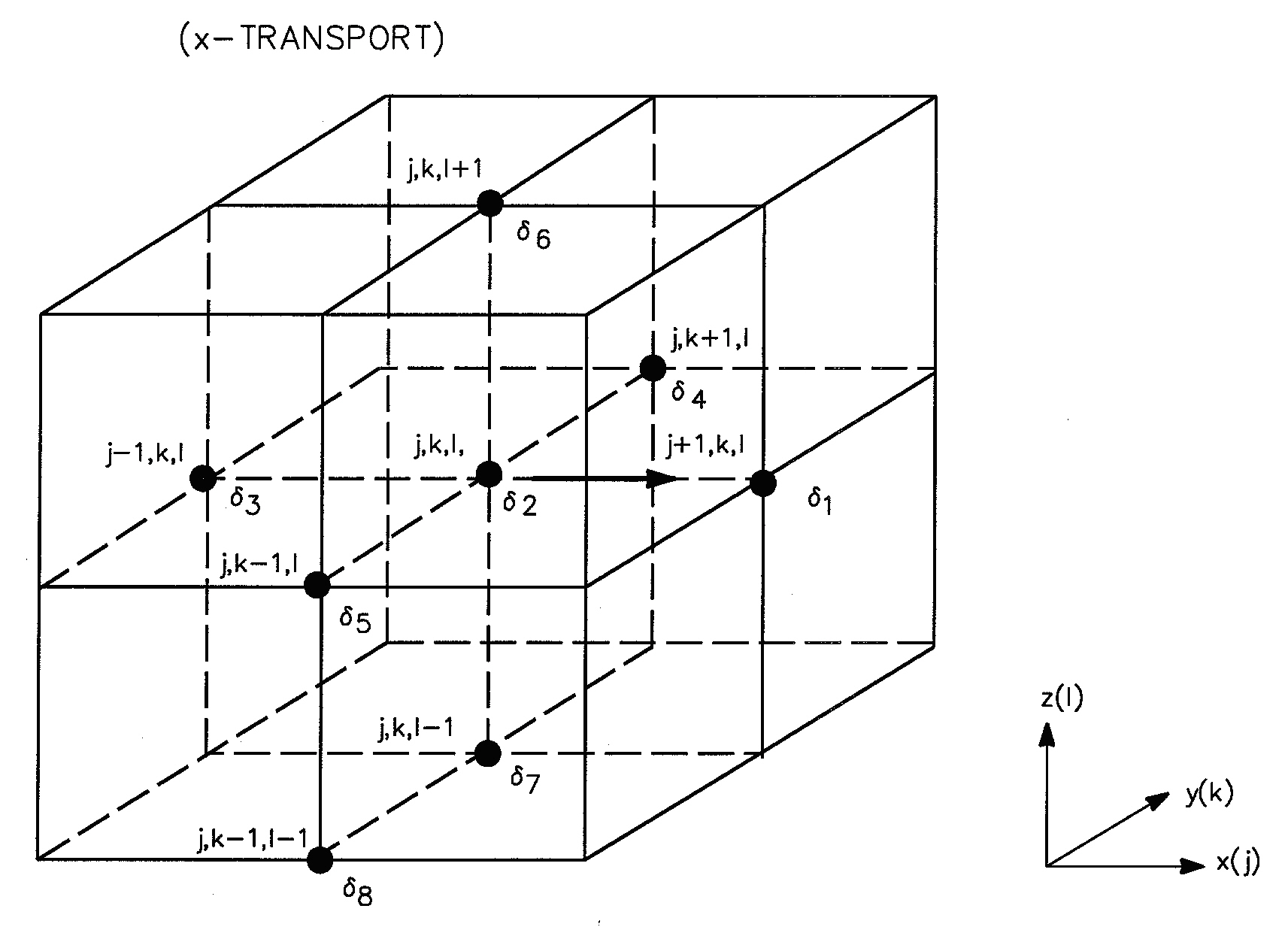
Figure 33.4        Location of interpolation weights for determination of concentrations at the location (j+½,k,l) - a grid boundary.

The dispersive transport can be derived in a similar way. With the finite differ­ence formulation of the dispersive transport components based on upstream differencing in concentrations and central differencing in dispersion coeffi­cients the transport in the x-direction can be expressed in the following man­ner:

(33.14)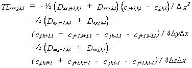   

The dispersive transports in the other directions are expressed in a similar way. The dispersive transports are incorporated in the weight functions so that the mass transports can be calculated in one step.