Solution scheme

The solution scheme applied for overland transport uses the same QUICK­EST scheme as in the saturated zone.It is a fully explicit scheme that using upstream differencing.

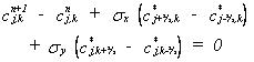
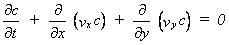
Neglecting the dispersion terms and the source/sink term and assuming that the flow field satisfies the equation of continuity and varies uniformly within a grid cell, the advection-dispersion equation can be written as

(33.30)   

and when written in finite difference form becomes

(33.31)   

where n denotes the time index.

In Eq. (33.31), s_x and s_y are the directional Courant numbers defined by

(33.32)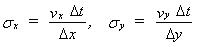   

and the c^*-terms are the concentrations at the surface of the control volume at time n. As these terms are not located at nodal points, they are interpolated from known concentration values by

(33.33)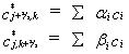   

The concentration c_i is the concentration around the actual point, for example (j-1,k) and the weights d_i and d_i are determined in such a way that the scheme becomes third-order accurate. The determination of the weights is demon­strated in Vested et al. (1992) and listed in Table 33.3. The other “boundary” concentrations are found in a similar way.

The locations of the weights are determined by the points that enter into the discretisation. Since the scheme is upstream centred, the weights are posi­tioned relative to the actual direction of the flow. This is outlined in more detail for in the saturated zone Solution Scheme (V1 p. 667) section.

The dispersive transport can be derived in a similar way. With the finite differ­ence formulation of the dispersive transport components based on upstream differencing in concentrations and central differencing in dispersion coeffi­cients, the transport in the x-direction can be written as

(33.34)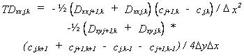   

The dispersive transport in the y direction is done in a similar way. The dis­persive transports are incorporated in the weight functions, so that the mass transports can be calculated in one step.