Irrigation Command Areas

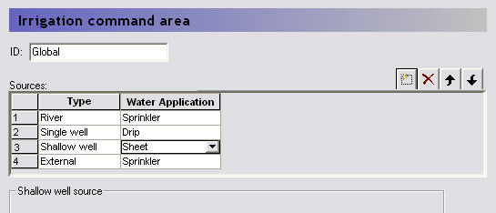
The Irrigation Command Areas are used to describe where the water comes from and how the irrigation water is applied to the model.

The Irrigation Command Area data item is divided into two dialogues. The first is the distribution dialogue for the Command Areas and the second is the Water source and Application method for each of the command areas.

Each source can also be limited by a licensed maximum amount of water in any period - License Limited Irrigation (V1 p. 257).

Using shp files

If you specify a shp file for the distribution of the command areas, then an extra dialogue will appear where you can specify a .dbf file to import all of the command area information. If you want to use this option, please email your local support center to obtain an example .shp and .dbf file combination.

Calculation sequence and shortage handling for SZ Linear Reservoirs

For each rank (no. of ranks = max no. of sources specified for any command area) and each Priority (usually only 1) do the following:

1.       Calculate the total demand of remote- and shallow well sources of the actual Rank and Priority from all baseflow reservoirs (1 & 2).

2.       Calculate a “supply factor” for each baseflow reservoir 1 & 2: If the demand is less than the storage of the actual reservoir, the supply factor is 1.0. Otherwise calculate a value between 0 and 1 = available storage / demand.

3.       Calculate the final irrigation from each source of the actual Rank and Pri­ority = calculated demand from actual baseflow reservoir 1 and/or 2 X corresponding supply factor.

4.       Subtract the final irrigation volumes from the available volume of each baseflow reservoir 1 & 2 and go to next rank and priority.

In the next SZ Linear Reservoir time step, the calculated irrigation volumes are subtracted from the baseflow reservoir storages (and depths), and the irrigation pumping is stored together with the other SZLR results for water balance calculation, etc.

The available volume of water in each baseflow reservoir is calculated as

(12.7)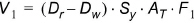   

(12.8)   

where V is the available volume of water, D_r is the depth of the reservoir, D_w is the depth to the water surface in the reservoir, S_y is the specific yield of the reservoir, A_T is the total surface area of the reservoir and F₁ is the fraction of infiltration that is added to the first Baseflow reservoir.

Water Source Types

The Sources table specifies the different sources available for irrigation for a single command area. The order of the sources in the table is also their prior­ity. For example, in the figure above, as long as there is sufficient water in the river, the irrigation water will be removed from the river. If the River falls below a specified level and/or discharge, then the irrigation water will be taken from the single well, and so on.   

River Sources

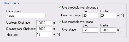
To use a river as a source of water, you must specify the MIKE Hydro River location to be used followed by the permitted river conditions that allow water to be removed. The River source actually has two conditions that can be used alone or combined.

River Name - The Branch name of the river source. This name must exist in the MIKE Hydro River model and it must be spelled correctly.

Upstream/Downstream Chainage - The upstream and downstream chain­age locations to use for the river source. MIKE SHE will use the com­bined volume of all the included river links as the storage volume. The abstraction from each river link is volume weighted based on the total volume of the contained and partial river links.

Max rate - This is the maximum extraction rate for the river. If more water is required for irrigation, then the next source will be activated.

Use threshold river discharge - If the flow rate in the river falls below the Stop value, then water will no longer be taken from the River. How­ever, if the flow rate in the river increases again and reaches the Restart value, the river source will be reactivated. The discharge threshold is applied at the upstream chainage location to ensure that the inflow to the river source area meets the minimum flow rate.

Use threshold river stage - If the water level in the river falls below the Stop value, then water will no longer be extracted from the River. However, if the water level in the river increases again and reaches the Restart value, the river source will be reactivated. The river stage threshold is applied at the downstream chainage to ensure that the minimum water level in the river source area is maintained.

If both threshold values are specified, then the most critical one is used, and the source will not restart until both are satisfied.

Note: There is no restriction on the number of river sources at a location. However, if the sources are located in the same model grid then a warning message will be printed to the projectname_preprocesssor_messages.log file. The sources will be merged, retaining the maximum threshold stages and the sum of the capacities. The preprocessor also checks the license applica­tion volume to make sure these are the same. If not, the preprocessor will stop with an error.

Single Well Sources

To use a well source in the model, you must specify the location and filter depth of the well. In a future release, this dialogue will be connected to the well database, but at the moment it is not.

X, Y -Pos - This is the X and Y map coordinates of the source well.

Max depth to water - this is the threshold value for the water depth in the well. If the water level in the well falls below this depth (as measured from the topography), the extraction will stop until the water level rises above the threshold.

Max rate - This is the maximum extraction rate for the well. If more water is required for irrigation, then the next source will be activated.

Top/Bottom of Screen - The depth of the top and bottom of the screen is used to define from which numerical layers water can be extracted. Pumping will stop if the water table falls below the bottom of the layer that contains the filter bottom.

There is no restriction on the number of wells at a location. However, if the wells are located in the same model grid, and have overlapping screen inter­vals, then a warning message will be printed to the projectname_preprocess­sor_messages.log file. The sources will be merged, retaining the maximum threshold depth, the sum of the capacities and the joint screening interval. The preprocessor also checks the license application volume to make sure these are the same. If not, the preprocessor will stop with an error.

In the linear reservoir groundwater method, multiple single wells are allowed in each baseflow reservoir. No warnings are given.

When the linear reservoir method is used, the screen interval is ignored and the water is pumped from the two baseflow reservoirs. The distribution between the two reservoirs is determined by the faction give in the Baseflow Reservoirs (V1 p. 304) dialogue. If the demand from one of the reservoirs exceeds the available water, the pumping will be reduced. The pumping rate at the other reservoir will not be increased to compensate.

Also in the Linear Reservoir method, the specified “max depth to water” for the actual command area and source is used. In other words, it is not using the “threshold depth for pumping” in the baseflow reservoir menu. Pumping is allowed when the depth to the water table is less than the specified threshold value at the start of the time step.

Shallow Well Sources

In many cases, farmers have several shallow wells for irrigation, most of which may not be mapped exactly. Especially in regional scale models, each grid cell could thus contain many shallow groundwater wells. In such cases, the Shallow Well source can be used to simply extract water for irrigation from the same cell where it is used, without having to know the exact coordi­nates of the wells. By specifying this option, one well is placed in each cell of the command area.

Note: A cell (i, j, layer) containing a shallow well cannot also have a single well specified in the same cell (i.e. the same cell and layer).

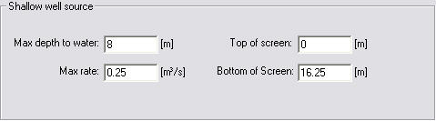
Max depth to water - this is the threshold value for the water depth in the well. If the water level in the well falls below this depth (as measured from the topography), the pumping will stop until the water rises above the threshold depth again.

Max rate - This is the maximum extraction rate for the shallow well in each cell. If more water is required for irrigation, then the next source will be activated.

Top/Bottom of Screen - The depth of the top and bottom of the screen is used to define from which numerical layers water can be extracted. Pumping will stop if the water table falls below the bottom of the layer that contains the filter bottom.

Shallow well sources are removed from baseflow Reservoir 1 if the Linear Reservoir groundwater method is used. The screen interval is ignored.

Note: Shallow wells can be located in cells containing single sources. The preprocessor will give a warning for such violations. Multiple shallow wells are not allowed in the same command area.

External Sources

In some case, the irrigation water can be from outside of the watershed being modelled. In this case, the only constraint is the maximum amount of water than can be extracted from the source.

Max rate - This is the maximum extraction rate for the source. If more water is required for irrigation, then the next source will be activated.

Water Application methods

There are three ways to apply the irrigation water in the model.

Sprinkler - If the water is applied as sprinkler irrigation, it is added to the pre­cipitation component.

Drip - If the water is applied as Drip irrigation, it is added directly to the ground surface as ponded water.

Sheet - If the water is applied as Sheet irrigation, then an additional data tree item is required to define where the water is to be added within the command area. The idea behind this option is that water is flooded onto one or more cells of the command area and then distributed to the adjoining cells as overland flow. The sheet irrigation is applied directly to the cells as ponded water.

All three methods are allowed in the Simple, sub-catchment based overland flow method. However, the sheet method does not really make sense if the subcatchment overland flow method is used.

License Limited Irrigation

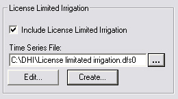
Sometimes, the total amount of irrigation water that a user can apply is limited by a license over a certain period (e.g. 10000 m³ / year). The license limited option, allows you to specify a dfs0 time series file with a time series of maxi­mum amounts. If the maximum amount is reached within the license period, then the irrigation will be stopped until the next license period, when it will be started again. The license period length is defined by the time steps in the specified dfs0 file.

During the simulation the license data is included in the calculation of the available water volume of each source. The module keeps track of the “actual available license volume”. Whenever this is reached or exceeded, the source will be closed until a new license period starts (or the end of the simulation). When a source is closed for this reason, a message is printed in the wm_print.log file.

Notes

·         The dfs0 file EUM Data Units (V1 p. 135) must be Water volume (m³ or other volume unit) and the time series-type must be Step Accumulated (V1 p. 149).

·         The specified volumes cover the period from the previous value (or start of simulation) until the date of the actual value.

·         The files may contain delete values. These are simply ignored. This makes it possible to include licenses for several sources in one file, even when the dates of the different source licenses differ.

·         An irrigation log file is included in the results output: projectname_Irriga­tionLicenseLog.dfs0.

·         This log file contains the “actual available license volume” of each source with license included, stored as instantaneous values at the end of every time step. This makes it easy to identify the periods where sources have been closed due to “license shortage”.

Note: Unused license volumes are NOT carried over to the next license period (use it or loose it !).