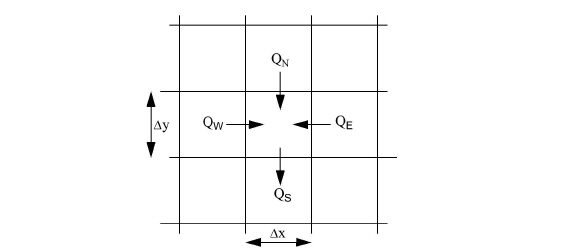
Consider the overland flow in a small region (see Figure 24.1) of a MIKE SHE model, having sides of length Dx and Dy and a water depth of h(t) at time t.
Figure 24.1 Square Grid System in a small Region of a MIKE SHE model
A finite-difference form of the velocity terms in Eq. (24.1) may be derived from the approximations
(24.9) 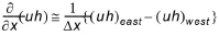
and
(24.10) 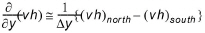
where the subscripts denote the evaluation of the quantity on the appropriate side of the square, and noting that, for example, Dx (uh)west is the volume flow across the western boundary
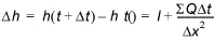
where
(24.12) 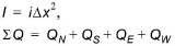
and where, i is the net input to overland flow in Eq. (24.1) and the Q's are the flows into the square across its north, south, east and west boundaries evaluated at time t.
Now consider the flow across any boundary between squares (see Figure 24.2), where ZU and ZD are the higher and lower of the two water levels referred to datum. Let the depth of water in the square corresponding to ZU be hU and that in the square corresponding to ZD to hD.
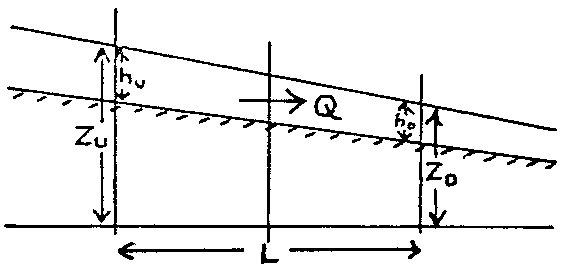
Figure 24.2 Overland flow across grid square boundary.
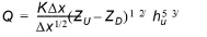
Equations (24.8a) and (24.8b) may be used to estimate the flow, Q, between grid squares by
where K is the appropriate Strickler coefficient and the water depth, hu, is the depth of water that can freely flow into the next cell. This depth is equal to the actual water depth minus detention storage, since detention storage is ponded water that is trapped in shallow surface depressions. Equation (24.13) also implies that the overland flow into the cell will be zero if the upstream depth is zero. The flow across open boundaries at the edge of the model is also calculated with Eq. (24.13), using the specified boundary water levels.
![]()