Numerical Solution of Richards Equation

MIKE SHE uses a fully implicit formulation in which the space derivatives of Eq. (28.7) are described by their finite difference analogues at time level n+1. The values of C(q) and K(q) are referred to at time level n+½. These are eval­uated in an iterative procedure averaging Cⁿ, Kⁿ with C^m, K^m respectively. C^m and K^m are calculated as a running average of the coefficients found in each iteration.

This solution technique has been found to eliminate stability and conver­gence problems arising from the non-linearity of the soil properties.

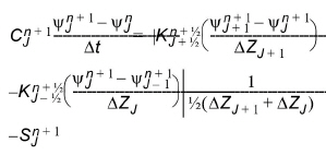
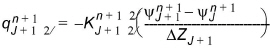
For an interior node, the implicit scheme yields the following discrete formula­tion of the vertical flow:

(28.8)   

where the subscript J refers to the spatial increment and the superscript n refers to the time increment. The vertical grid system for a soil column is shown in Figure 28.1. Similar to Eq. (28.8) the discrete form of Eq. (28.1) gives

(28.9)   

The soil property K is centred in space using the arithmetic mean:

(28.10)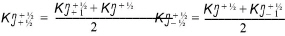   

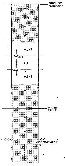
Figure 28.1        Vertical Discretisation in the Unsaturated Zone.

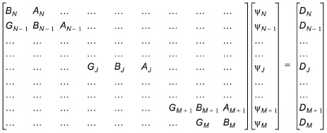
Eq. (28.9) involves three unknown values at time n+1 and one known value at time n for each node. Written for all nodes with reference to Figure 28.1, a system of N-M+1 equations with N-M+1 unknowns is obtained. The system of equations forms a tri-diagonal matrix:

(28.11)   

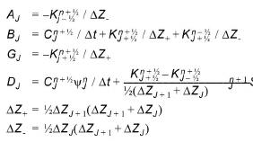
The J'th row in the matrix is

(28.12)   

where

(28.13)   

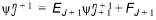
The solution to the matrix system Eq. (28.11) is solved by Gaussian elimina­tion. Assuming that  and can be related in the following recur­rence relation

(28.14)   

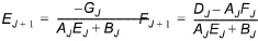
The E_J+1 and F_J+1 can be calculated by combining Eqs. (28.12) and (28.14) as follows:

(28.15)   

Given the boundary conditions at the bottom and top nodes, y is computed for all nodes in a double sweep procedure:

1.       E and F values are calculated from Eqs. 28.13 and 28.15 for all nodes from bottom-to-top in a E, F-sweep.

2.       y is then calculated from Eq. 28.14 for all nodes in a top-to-bottom sweep.

Briefly, the iterative procedure within each time step is

1.       the final result at time n (i.e.  and ) is used for the initial estimate of  and for the first iteration,

2.       then the following convergence criteria is checked for every node after each iteration, i

(28.16)               

(28.17)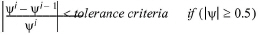               

3.       if this convergence criteria is satisfied then a solution at the current time level (i.e. n+1) has been found.

4.       if the criteria is not fulfilled then  and  are updated for the next iteration by

(28.18)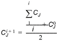   

(28.19)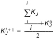